 FLIMKit
Plugins / FLIMKit / Step by Step Guide · edit on GitHub
Step-by-Step Guide
A worked analysis of one field of view, Ado_1.ptu, from opening the file to exporting the maps, followed by a project folder with a z-stack, the tile stitching form, and a list of every file FLIMKit reads and writes. Every screenshot is the desktop GUI running from source (v0.13.5 plus the commits after it), and every number quoted was produced by those runs. Your numbers will differ with your data and your machine IRF, but the order of the steps and the reasons for each setting carry over.
Ado_1.ptu is a single 1024 x 1024 px field of view: 1,714,555 photons in channel 1, 529 TCSPC bins of 96.97 ps, a 19.505 MHz laser (51.27 ns period) and 127.5 s of acquisition.
Step 1: Open the file
Start the GUI (python main.py, or the compiled app) and stay in Single FOV Fit mode.
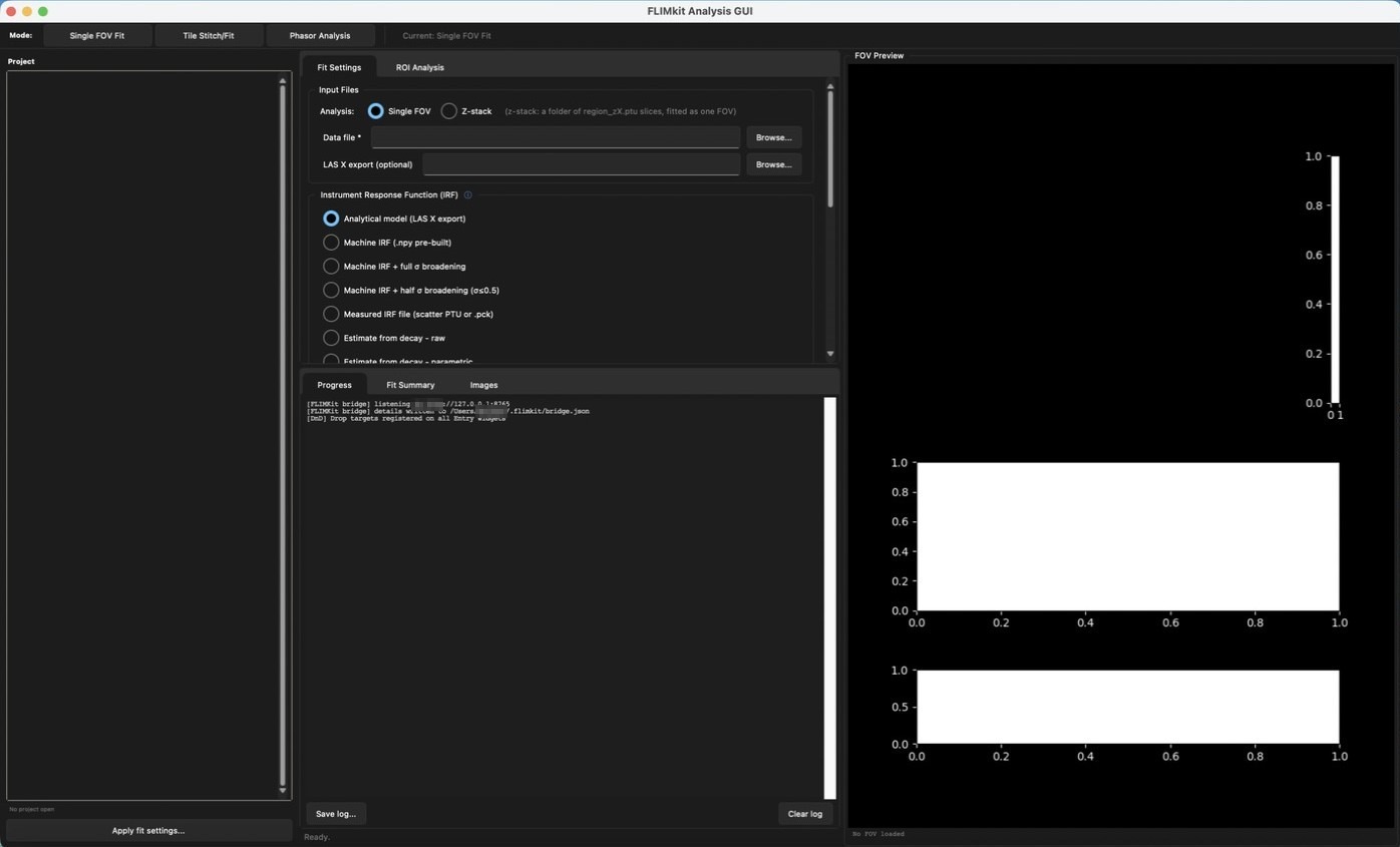
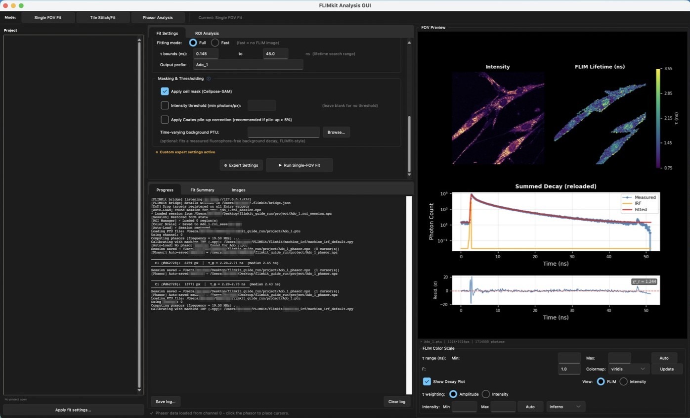
The window has four areas. The Project list on the left fills when you open a folder (Step 13). The settings form sits in the middle, with the Progress log, Fit Summary and Images tabs underneath. The FOV Preview on the right shows the intensity image, the lifetime map and the summed decay.
Input Files:
| Option | What it does |
|---|---|
| Analysis: Single FOV | One file, one field of view. |
| Analysis: Z-stack | A folder of region_zX.ptu slices fitted as one field of view (Step 14). |
| Data file | The FLIM file. Any format in Supported Input Formats works. Browse, type the path, or drag the file onto the box. |
| LAS X export (optional) | The .xlsx (or delimited text) exported from the LAS X FLIM window for this same file. It is only needed for the Analytical model IRF, and it lets you compare against the LAS X fit. |
Load Ado_1.ptu. The preview draws the intensity image and the summed decay straight away, and the status line under the preview gives the image size and photon count.
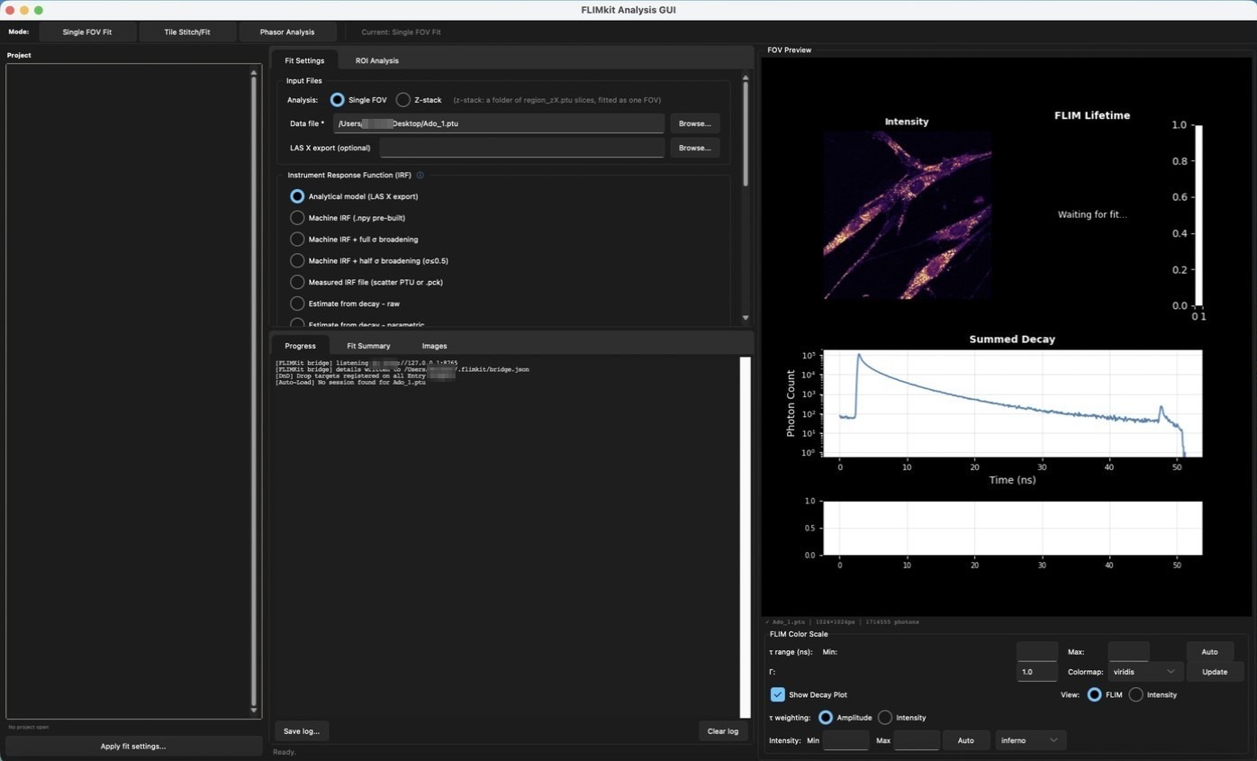
If a Ado_1.roi_session.npz already sits next to the file, FLIMKit restores the last fit, the ROIs and the form settings from it instead of starting clean. The log says [Auto-Load] No session found when there isn't one.
Look at the decay before you change anything. This one rises at about 2.6 ns, decays over roughly three decades, and has a small peak at about 47 ns. That peak is the start of the next laser period, and FLIMKit finds it and cuts the fit window short of it on its own (Step 6).
Step 2: Choose the IRF
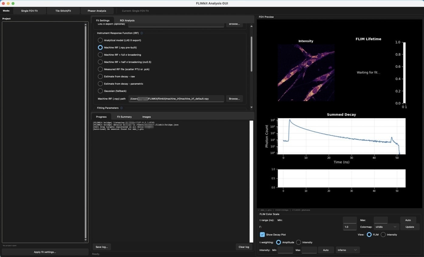
The instrument response function is the largest single source of systematic error in a reconvolution fit, and it matters most for the shortest component. The ⓘ next to each section heading opens the same explanations inside the app.
| Option | When to use it |
|---|---|
| Analytical model (LAS X export) | Builds the IRF from the LAS X export named in Input Files. The default for FALCON data when you have the export for this file. |
| Machine IRF (.npy pre-built) | A stored IRF for your microscope, built once from matched pairs (Machine IRF Setup). Use it when the optical path hasn't changed since it was built. |
| Machine IRF + full σ broadening | The same stored IRF, which the fit may broaden with a Gaussian of up to 3.0 bins. For when the stored IRF is narrower than the real response, after a change of objective or pinhole for example. |
| Machine IRF + half σ broadening (σ≤0.5) | Broadening capped at 0.5 bins. For a stored IRF that is close, where a free σ would start absorbing the decay. |
| Measured IRF file (scatter PTU or .pck) | An IRF recorded alongside the sample from a scattering solution or a reflective surface. The most defensible choice when you have one. |
| Estimate from decay - raw | Takes 21 bins around the decay peak as the IRF. A last resort: it can't separate the instrument from the fastest part of the decay, so short lifetimes come out long. |
| Estimate from decay - parametric | Fits a pulse shape to a 1.5 ns window around the peak. Smoother than raw, with the same bias. |
| Gaussian (fallback) | A Gaussian of the configured width. |
The Machine IRF path box appears under the options when a machine IRF method is picked, filled with your default. The default can be changed in File > Preferences... > Files (Machine IRF Setup). For Ado_1.ptu I used Machine IRF, since there is no LAS X export for this file.
Step 3: Set the fitting parameters
| Option | What it does |
|---|---|
| Fit model: n-exp | A sum of 1, 2 or 3 discrete exponentials convolved with the IRF. The right choice for most samples. |
| Fit model: Gaussian dist. | One continuous distribution of lifetimes, reported as a centre and a width. For a fluorophore in a heterogeneous environment where a discrete fit needs too many components. Slower, since each evaluation integrates over a 200-point lifetime grid. |
| Fit model: Lorentzian dist. | The same with heavier tails, so a small sub-population far from the centre doesn't drag the centre towards it. |
| Fit model: n-exp tail | Discrete exponentials fitted past the decay peak with no IRF. Fast, and the IRF drops out as a source of error, but components shorter than about the IRF width come out biased. The IRF section is hidden when this is picked. |
| Components | 1, 2 or 3 for n-exp and tail, or 1 (unimodal) / 2 (bimodal) for the distributions. Start low and add a component only when the residuals show structure (Step 6). |
| Fitting mode: Full | Fits the summed decay, then every pixel. This is what makes the lifetime map. |
| Fitting mode: Fast | The summed decay only. Seconds instead of minutes, with no map. Use it to check the IRF, the model and the component count first. |
| τ bounds (ns) | The lower and upper bounds on the fitted lifetimes (0.145 and 45 ns by default). The part of the decay that is fitted is set separately, in Expert Settings. |
| Output prefix | Where the output files go and what they're called. It fills with the file name, so outputs land next to the data. A bare name is placed in the data folder; a full path is used as it is. |
Step 4: Masking and thresholding
| Option | What it does |
|---|---|
| Apply cell mask (Cellpose-SAM) | Segments cells in the intensity image and fits only inside them, so background pixels don't add noise-dominated lifetimes to the statistics. It runs on the GPU when there is one. Needs the segmentation extra. |
| Intensity threshold (min photons/px) | Skips pixels below this count. Blank means no threshold. |
| Apply Coates pile-up correction | Corrects the early-photon bias at high count rates. The log prints the photons per pulse at the start of each fit: tick this above about 5%. The corrected decay is no longer Poisson, so χ²_r is unreliable with it on, though the lifetimes are not. |
| Time-varying background PTU | A separate acquisition of a fluorophore-free region (medium, buffer). Its decay shape is fitted as a scaled background instead of a flat offset (Time-varying background correction). |
Ado_1.ptu ran at 0.0007 photons per pulse (0.07%), so pile-up correction stays off. I left the mask off for the first fits to show what it changes in Step 8.
Step 5: Expert settings
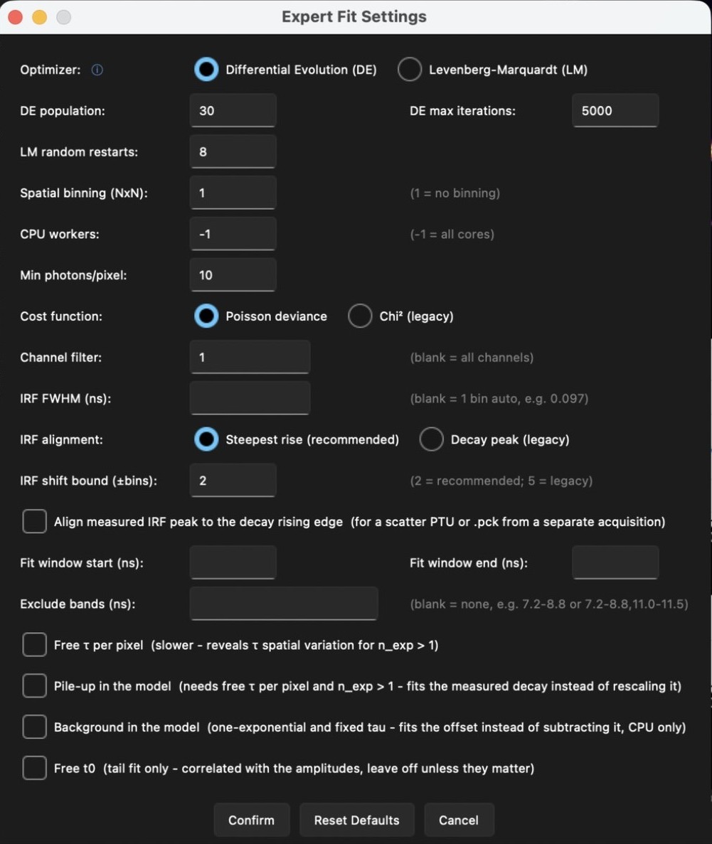
Expert Settings opens a dialog shared by the single FOV and tile pipelines. When anything in it differs from the defaults, an orange "Custom expert settings active" line appears above the run button.
| Option | What it does |
|---|---|
| Optimizer: Differential Evolution (DE) | A global search over the bounded parameter space with a Levenberg-Marquardt polish at the end. It doesn't depend on a starting guess. The default. |
| Optimizer: Levenberg-Marquardt (LM) | A local fit from several starting points. Much faster, and it can miss the global minimum on a multi-exponential decay with few restarts. |
| DE population / DE max iterations | DE search size (30 and 5000). |
| LM random restarts | Number of LM starting points (8). |
| Spatial binning (NxN) | Sums N x N pixels before the per-pixel fit. 1 is no binning. See Step 7. |
| CPU workers | Cores for DE. -1 uses all of them. The compiled app is limited to 1. |
| Min photons/pixel | Pixels below this count are left out of the per-pixel fit (10). |
| Cost function | Poisson deviance (default) or the legacy Neyman χ². Poisson is correct for photon counts, above all at low counts. |
| Channel filter | Detector channel. Blank uses all channels. |
| IRF FWHM (ns) | Width for the estimated and Gaussian IRFs. Blank is one TCSPC bin. |
| IRF alignment | Where the IRF is anchored against the decay. Steepest rise (default) or the legacy decay peak. |
| IRF shift bound (±bins) | How far the fit may shift the IRF in time. 2 is recommended; 5 is the old default. |
| Align measured IRF peak to the decay rising edge | For a scatter PTU or .pck recorded in a separate acquisition, whose time zero won't match the sample's. |
| Fit window start / end (ns) | The part of the decay that is fitted. Blank lets FLIMKit choose from the IRF onset and the end of the period. |
| Exclude bands (ns) | Stretches of the decay to leave out, such as a reflection peak, written 7.2-8.8 or 7.2-8.8,11.0-11.5 (Fit window and exclusion bands). |
| Free τ per pixel | Lets lifetimes float in every pixel instead of locking them to the summed fit. Slower, and it shows spatial variation in τ when n_exp > 1. The accelerator plugin can speed it up a lot, but nothing needs it. |
| Pile-up in the model | Fits pile-up as part of the model instead of rescaling the decay. Needs free τ per pixel and n_exp > 1. |
| Background in the model | Fits the offset instead of subtracting it. One exponential with fixed τ, CPU only. |
| Free t0 | Tail fits only. Lets the start time float, which correlates with the amplitudes. |
| Bootstrap errors / resamples | On by default, with 25 resamples. Refits the summed decay 25 times on resampled copies of the data to measure the ± on each lifetime (Parameter uncertainties). It adds about 35 s to a 1-exponential fit and a minute to a 3-exponential one, so untick it for quick trial fits. |
| Confirm / Reset Defaults / Cancel | Apply, restore the defaults, or close without changes. |
For Ado_1.ptu I left everything at the defaults until Step 7.
Step 6: Run a fast fit first
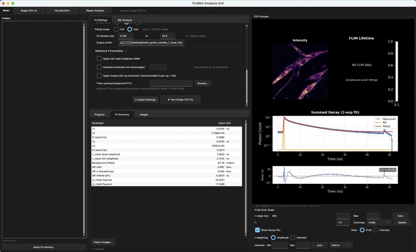
With Fast mode and 2 components, Run Single-FOV Fit took a few seconds.
The Progress log records every choice the fit made, so it's the first place to look when a result seems wrong.
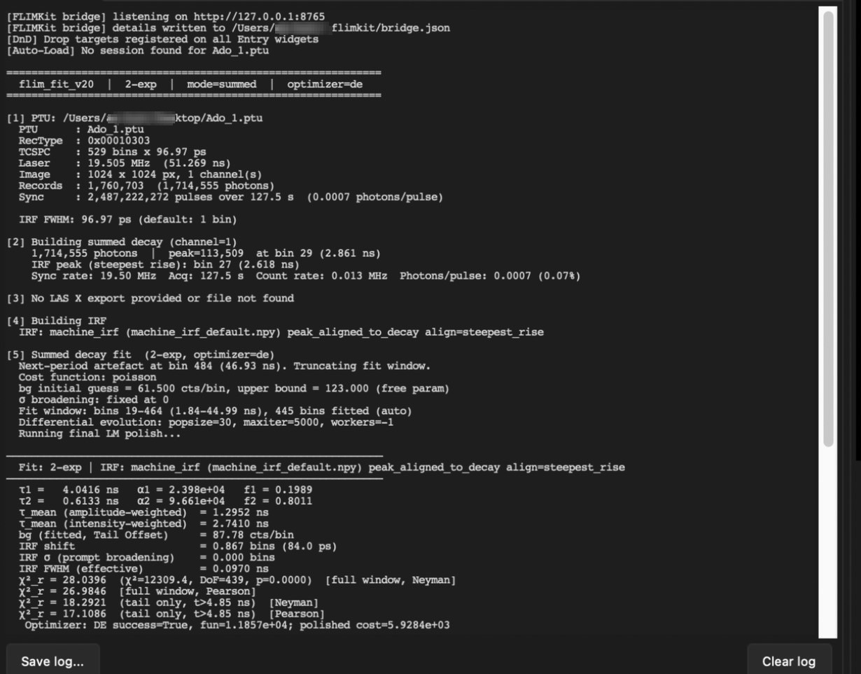
Section [1] reads the file header, and section [2] gives the count rate and photons per pulse used to decide on pile-up correction. Section [5] shows the fit window chosen: here FLIMKit found the next-period artefact at bin 484 (46.93 ns) and fitted bins 19-464 (1.84-44.99 ns) automatically.
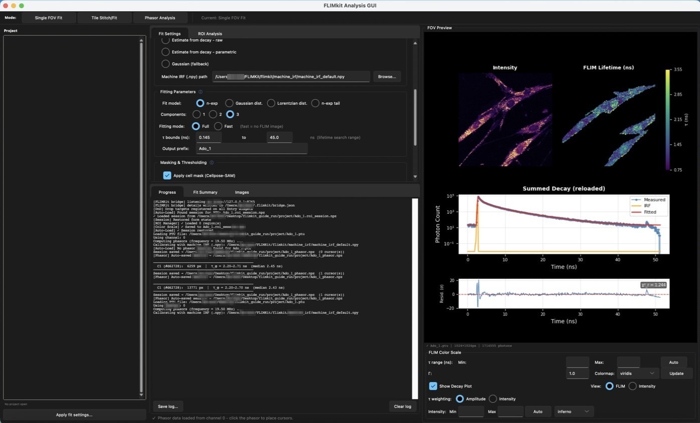
The 2-exponential result was τ₁ = 4.04 ns and τ₂ = 0.61 ns with χ²_r(tail) = 18.29, and the residuals have a clear wave across the first 20 ns. That structure means the model is missing something. Changing to 3 components and running again dropped χ²_r(tail) to 1.53 and flattened the residuals, so I kept three. A lower χ² on its own doesn't justify an extra component, since more parameters always fit better. Check that the new lifetimes are physically distinct and that the residuals improved.
Step 7: Full fit and binning
With 3 components, switch Fitting mode to Full and run again. A progress window counts the pixels as they're fitted.
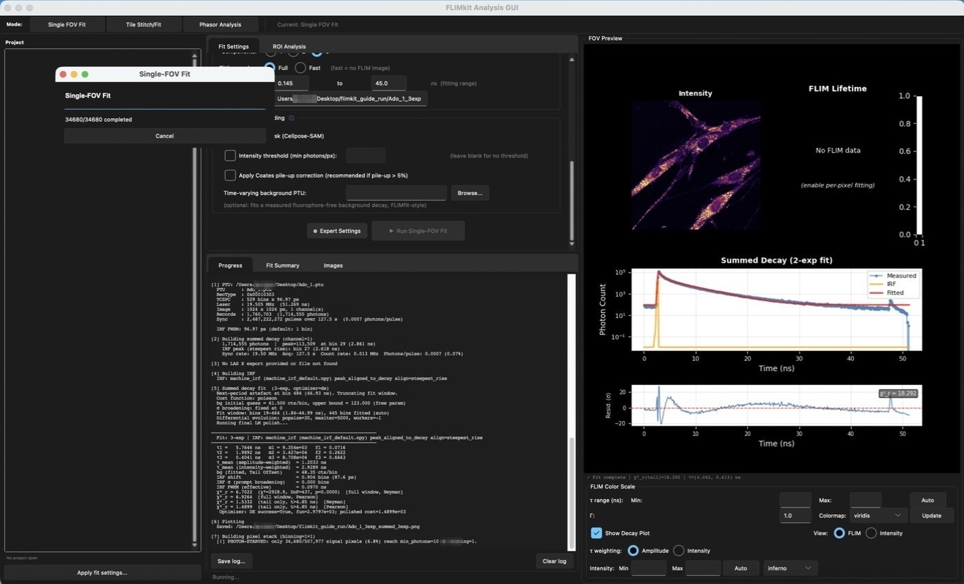
At binning 1 only 34,680 of 507,977 signal pixels (6.8%) reached the 10-photon minimum, which the log flags as PHOTON-STARVED. When most of the image is starved, FLIMKit says so when the fit finishes and suggests a binning.
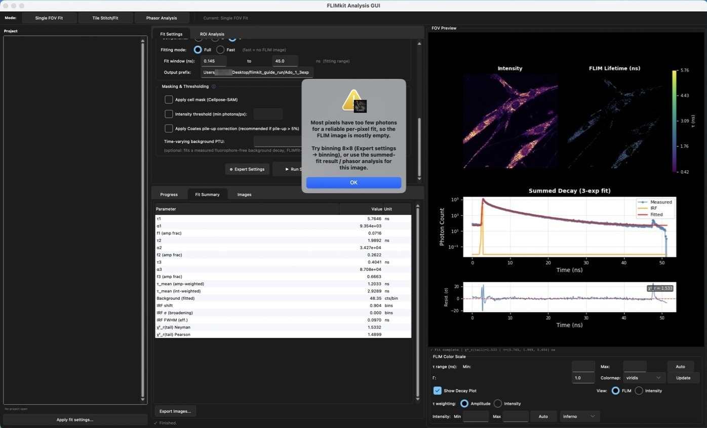
Binning sums an N x N block of pixels into one decay before fitting, trading resolution for photons per pixel. With Spatial binning set to 8 in Expert Settings, the map filled in.
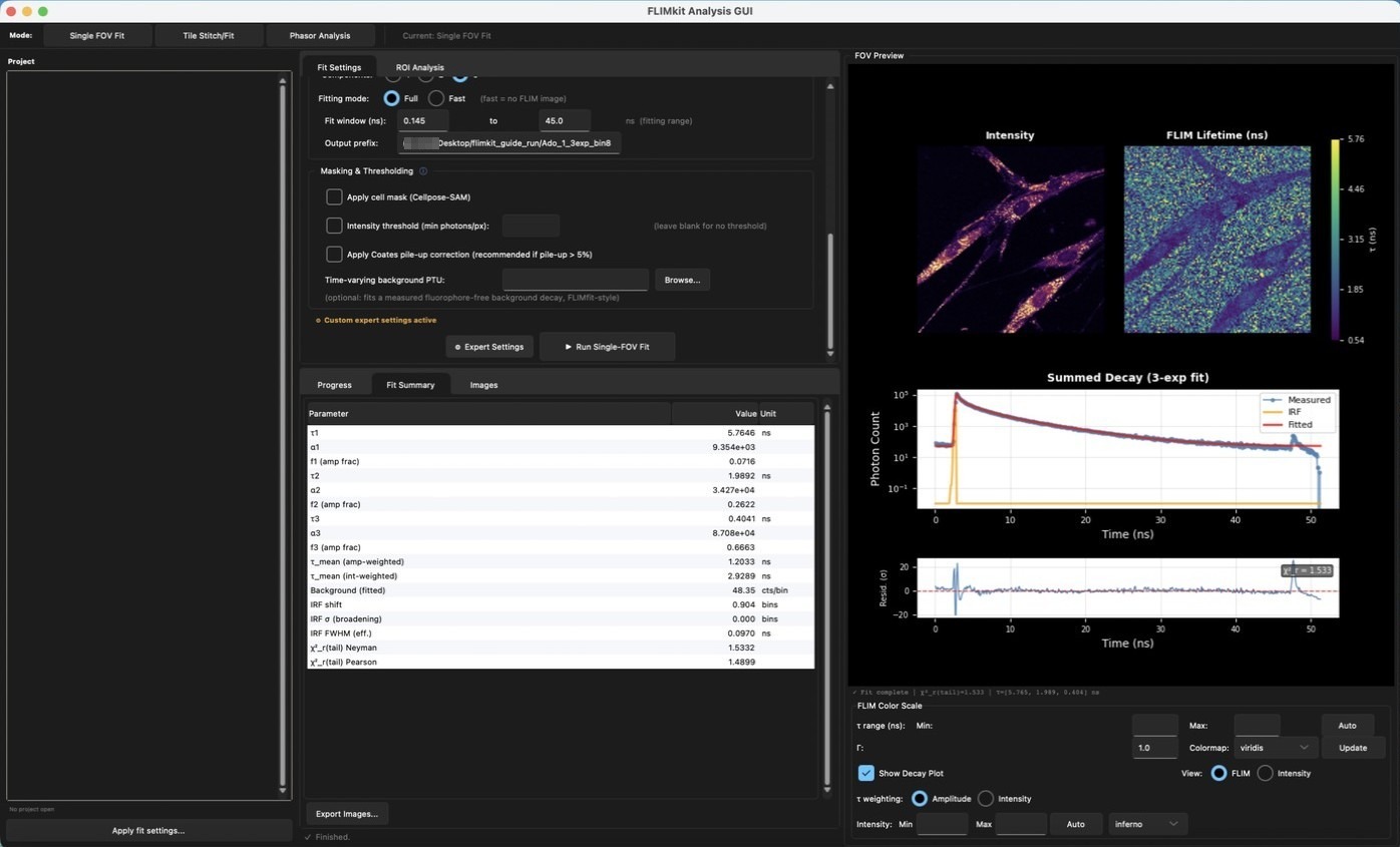
The per-pixel fit keeps the summed-fit lifetimes and fits only the amplitudes in each pixel, unless Free τ per pixel is on. The map is the amplitude-weighted mean lifetime per pixel. The background between the cells now fills with noise-dominated values, which the next step removes.
Step 8: Mask out the background
Tick Apply cell mask (Cellpose-SAM) and run again.
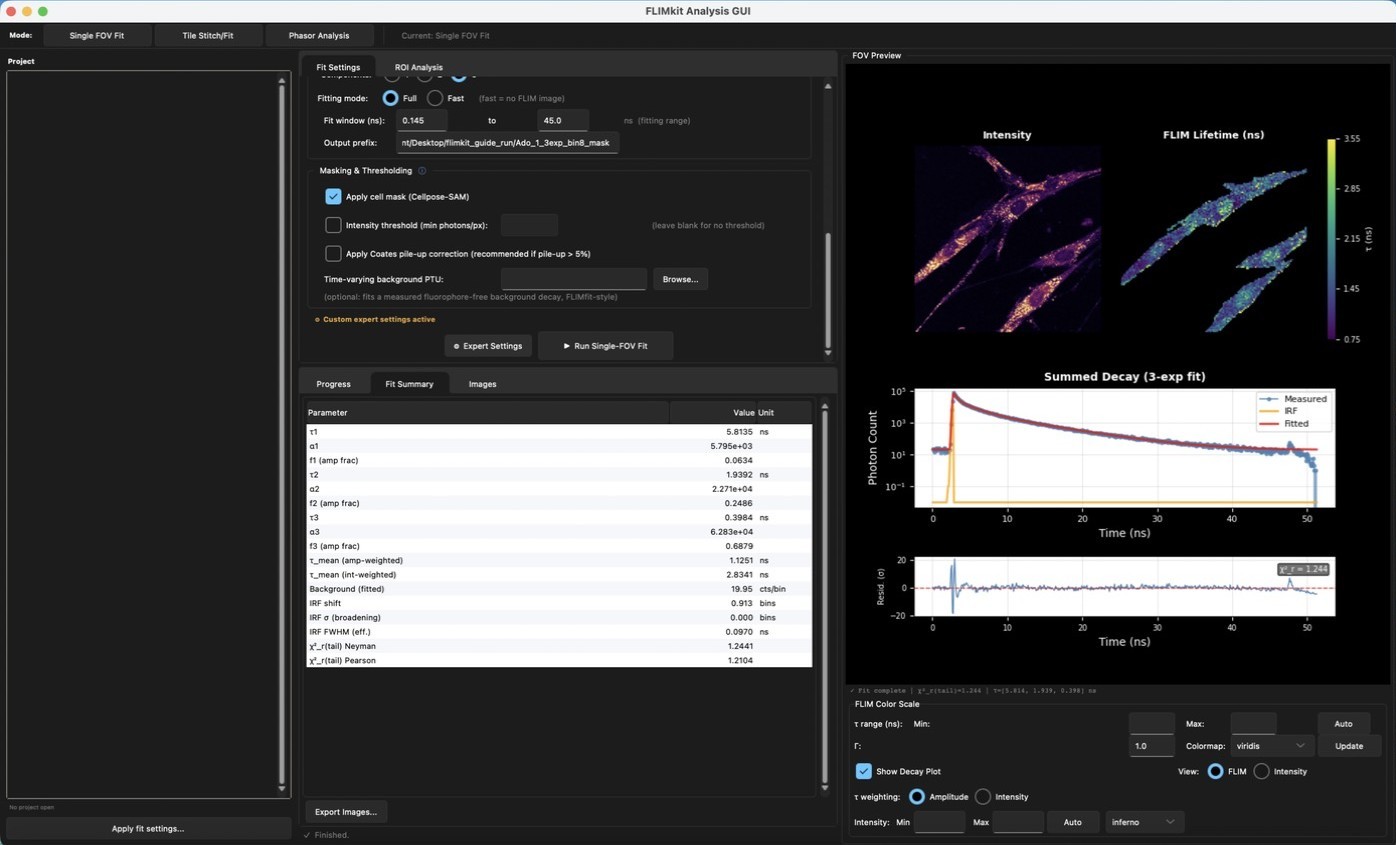
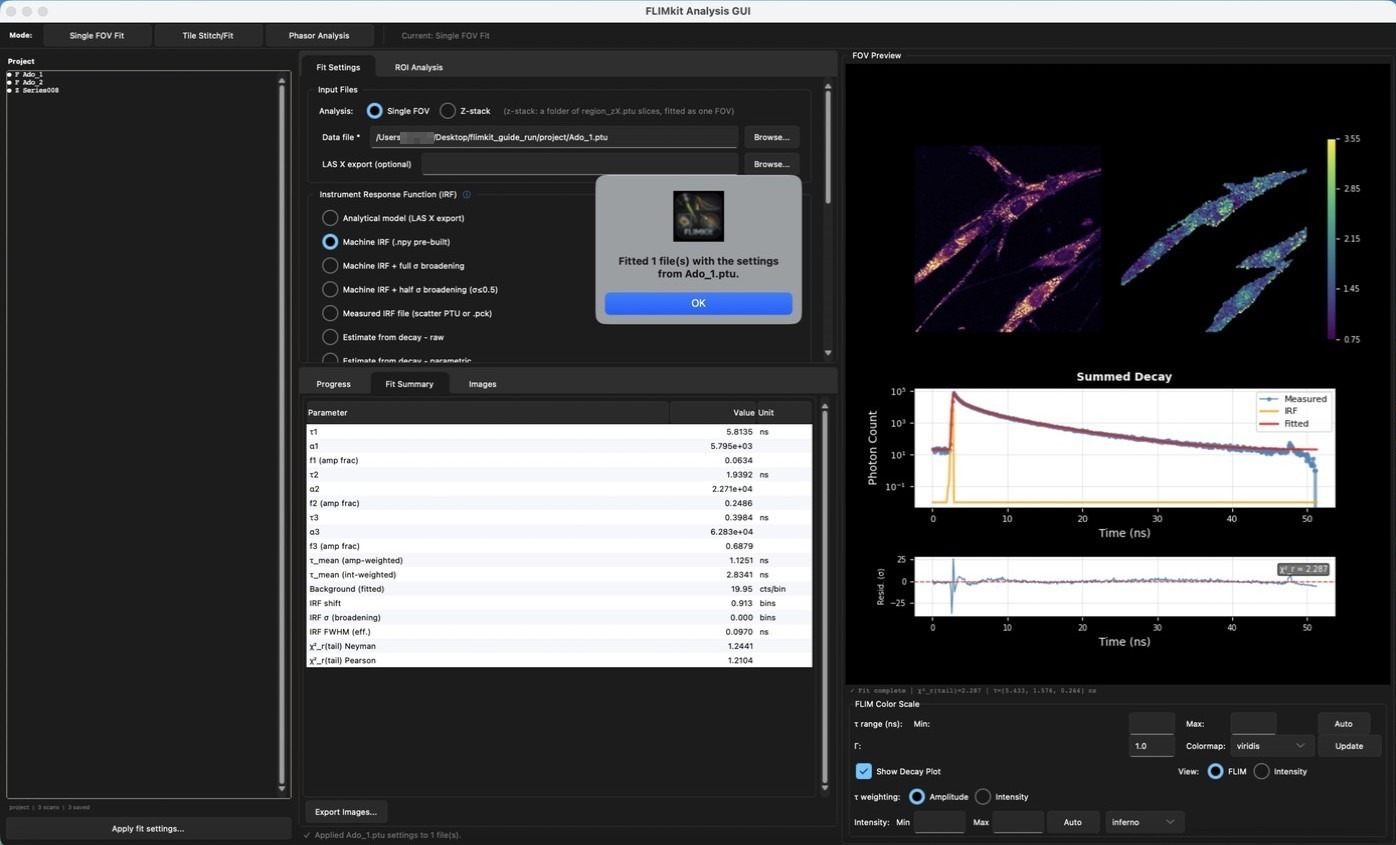
The map now covers the segmented cells only. The summed decay is built from those pixels too, so the global fit changes with it: τ = 5.81, 1.94 and 0.398 ns and χ²_r(tail) = 1.244. Cellpose missed part of one cell at the top left here, so check the mask (saved as <prefix>_cell_mask.png) before trusting the per-cell statistics.
Fit Summary tab, row by row:
| Row | Meaning |
|---|---|
| τ1, τ2, τ3 | Component lifetimes from the summed fit, in ns. |
| τ1 ± (1σ), τ2 ± (1σ), τ3 ± (1σ) | Standard error of each lifetime from the fit curvature, in ns. See Fit Diagnostics. |
| τ1 ± (bootstrap), ... | Standard deviation of each lifetime over the bootstrap refits. Trust this one over the curvature error when they disagree. |
| α1, α2, α3 | Component amplitudes, in counts. |
| f1, f2, f3 (amp frac) | Amplitude fractions, αᵢ / Σα. |
| τ_mean (amp-weighted) | Σαᵢτᵢ / Σαᵢ. Weighted towards the short, high-amplitude components (1.125 ns here). |
| τ_mean (int-weighted) | Σαᵢτᵢ² / Σαᵢτᵢ. Weighted towards the long components, closer to what a phasor or a mean arrival time gives (2.834 ns here). |
| τ_mean ± (1σ) / ± (bootstrap) | Error on each mean lifetime, from the curvature and from the bootstrap. |
| Bootstrap resamples | How many resampled refits the bootstrap errors came from. |
| Background (fitted) | Constant offset per bin. |
| IRF shift | How far the IRF was moved to match the decay, in bins (0.913 bins, about 88 ps). |
| IRF σ (broadening) | Extra Gaussian width. 0 unless a broadening IRF method is used. |
| IRF FWHM (eff.) | Effective IRF width after any broadening. |
| χ²_r(tail) Neyman / Pearson | Reduced χ² over the tail of the decay, kept for comparison with LAS X. See Fit Diagnostics. |
| ⚠ rows | A lifetime the data can't pin down: more than 10% error, or two lifetimes correlated beyond |r| = 0.95. |
Running the same fit twice gives identical numbers, since both optimisers are seeded. I refitted Ado_1 from a project folder in Step 13 and every value matched to the last digit.
The figures the fit saves
Every fit saves its figures next to the output prefix without being asked. These are from the masked 8 x 8 fit above.
<prefix>_summed_<n>exp.png is the summed fit.
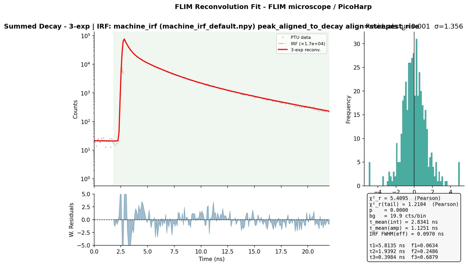
| Part | What it shows |
|---|---|
| Top left | The summed decay (grey dots), the IRF scaled to a tenth of the decay peak (orange, the scale factor is in the legend) and the fitted model (red), on a log axis. The green band is the fit window. Only the first 22 ns are drawn, so a window running further than that is cut off on the plot but not in the fit. |
| Bottom left | Weighted residuals across the fit window, clipped to ±5. A good fit scatters evenly around zero. A wave, like the one the 2-exponential fit in Step 6 left, means the model is missing something. |
| Top right | Histogram of the same residuals, with their mean and SD. It should be a single peak at zero with an SD near 1. The residuals are clipped at ±5, so spikes at the edges are the points that fell outside that range. |
| Bottom right | χ²_r over the fit window and χ²_r(tail), background, both mean lifetimes, the effective IRF width, and each τᵢ with its amplitude fraction fᵢ. The χ² values here are Pearson, so they differ from the Neyman χ²_r(tail) on the preview's residual plot: 1.2104 here against 1.244. The Fit Summary tab lists both. |
<prefix>_pixelmaps_<n>exp.png is the per-pixel fit, only written by Full fits.
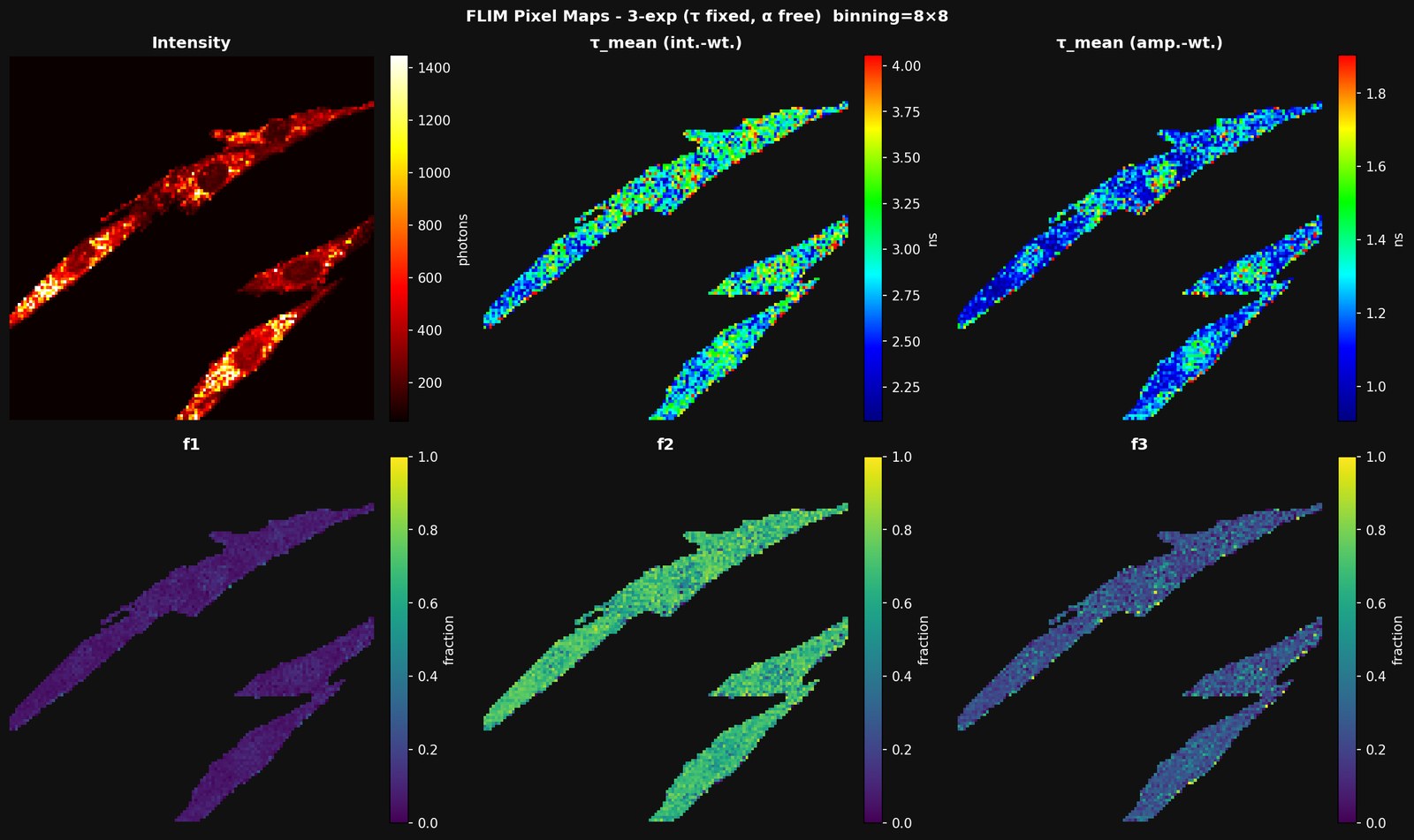
The top row is the photon count per pixel, the intensity-weighted mean lifetime and the amplitude-weighted mean lifetime. The bottom row is the amplitude fraction of each component, on a fixed 0 to 1 scale. The lifetime and intensity colour ranges run from the 2nd to the 98th percentile of the fitted pixels, so they won't match the range set in the preview, and unmasked background shows up as noise the same way it does on screen.
<prefix>_lifetime_hist_<n>exp.png is the distribution of per-pixel lifetimes.
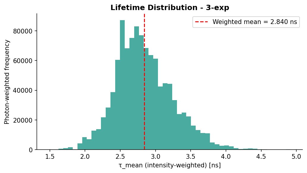
Each pixel's intensity-weighted mean lifetime, weighted by its photon count, with the weighted mean as a dashed line: 2.840 ns here, against 2.834 ns from the summed fit. The preview map shows the amplitude-weighted lifetime by default, so the histogram and the map aren't showing the same quantity.
<prefix>_cell_mask.png is the Cellpose mask at the full image resolution, white for the pixels kept. Check it against the intensity image before trusting per-cell numbers.
The PNG export in Step 11 writes separate figures: <scan>_summed_decay.png is the decay, IRF and fit from the preview over the whole time range, without residuals.
Step 9: Adjust the display
The FLIM Color Scale panel under the preview changes the picture, never the fitted values.
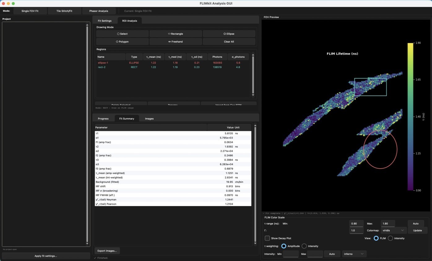
| Control | What it does |
|---|---|
| τ range Min / Max, Auto, Update | Colour limits in ns. Auto sets them to the 2nd and 98th percentiles of the map (0.90-1.90 ns for Ado_1). Type values and press Update to set them yourself. Values outside the range are clamped, not removed. |
| Γ | Gamma on the colour scale. 1.0 is linear. |
| Colormap | Colour map for the lifetime image. |
| Show Decay Plot | Hides the decay and residuals so the images get the whole panel. |
| View: FLIM / Intensity | With the decay plot hidden, which of the two images fills the panel. |
| τ weighting: Amplitude / Intensity | Recomputes the map as the amplitude- or intensity-weighted mean lifetime from the stored per-pixel amplitudes. No refit. |
| Intensity: Min / Max, Auto, colormap | The same for the intensity image. |
The colour scale is saved into the session file, so it comes back when the file is reopened.
Step 10: Measure regions of interest
Open the ROI Analysis tab, pick a drawing mode and drag on either image.
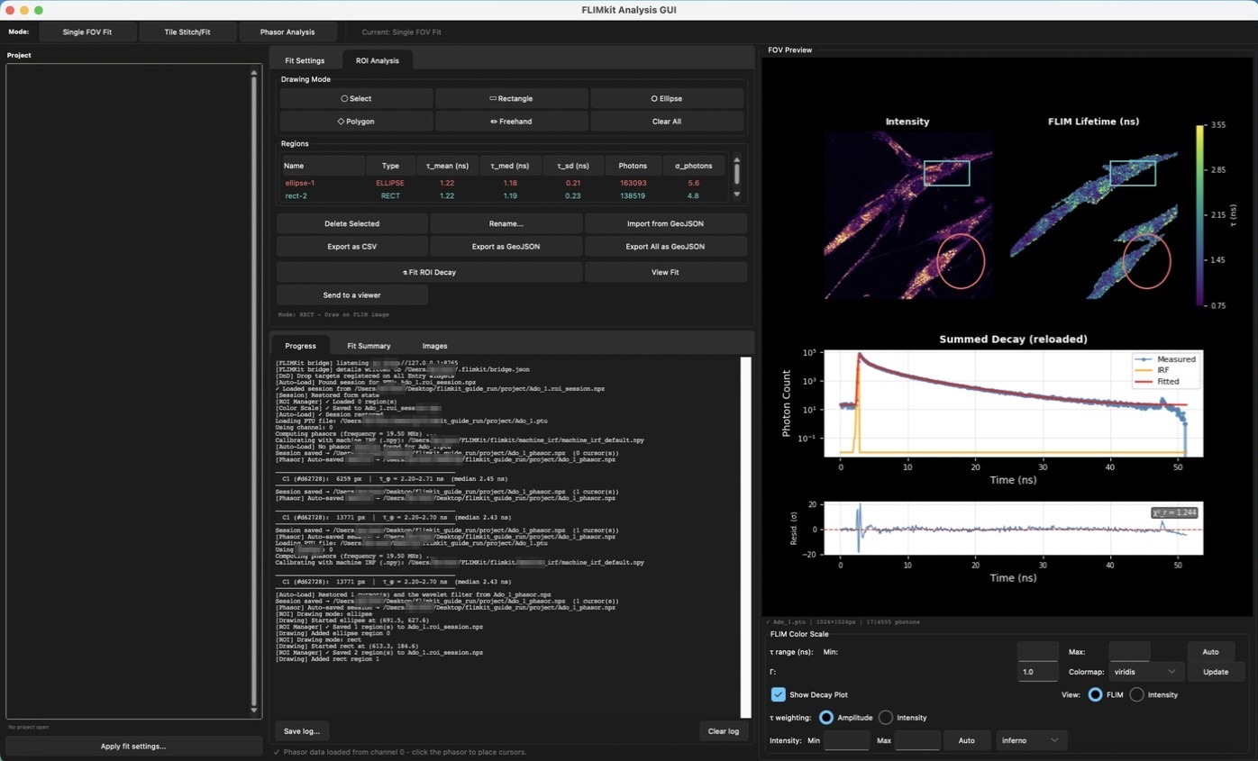
| Control | What it does |
|---|---|
| Select | Click a region on the image to select it. |
| Rectangle / Ellipse | Drag a box. |
| Polygon | Click the vertices, then right-click to close the shape (three points minimum). |
| Freehand | Draw the outline. |
| Clear All | Removes every region. |
| Delete Selected / Rename... | Act on the region selected in the list. |
| Import from GeoJSON | Loads regions drawn elsewhere, QuPath for example. Only the outer boundary of each shape is kept, so holes are lost. |
| Export as CSV | The Regions table as a spreadsheet. |
| Export as GeoJSON / Export All as GeoJSON | The selected or all regions, with their statistics, for QuPath. |
| Fit ROI Decay / View Fit | Fits the summed decay of the selected region(s) on its own (Per-ROI decay fitting). |
| Send to a viewer | Added by the flimkit-bridge plugin. Checks that a viewer such as QuPath has connected and says which images it is being served (FLIMKit Bridge). |
The table gives, per region, the mean, median and standard deviation of the pixel lifetimes and the photon count. The ellipse over the lower cell gave τ_mean = 1.22 ns (median 1.18, SD 0.21) from 163,093 photons, and the rectangle over the upper cell 1.22 ns (median 1.19, SD 0.23) from 138,519. Regions are written to the session file as soon as they're drawn.
Fit ROI Decay re-fits a region from the raw file rather than taking values from the whole-FOV fit. It sums every photon inside the outline at full resolution, so the FOV fit's binning, photon threshold and background mask don't apply to it. It reuses the IRF from the last FOV fit. If there isn't one it falls back to a 0.2 ns Gaussian on the decay peak, and the IRF label in the results window says which was used. The FOV fit and the lifetime map are left as they were.
Step 11: Export
Export Images..., under the Fit Summary table, saves the images shown in the preview.
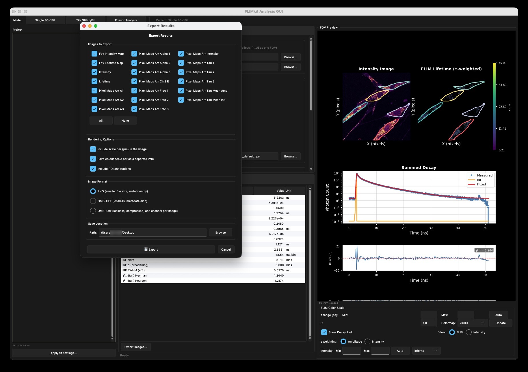
| Option | What it does |
|---|---|
| Images to Export | The maps the fit produced. After a fresh fit that is Intensity and Lifetime. A fit reopened from its session, as here, lists every map the session holds. PNG and OME-TIFF write Intensity and Lifetime; OME-Zarr writes every ticked map. All / None tick or clear them. |
| Include scale bar (µm) in the image | Draws a µm scale bar in the bottom right corner of the PNGs. The pixel size comes from the file, 0.189 µm for Ado_1.ptu, so the bar was 20 µm. A file with no pixel size gets no bar, and the export says so when it finishes. |
| Save colour scale bar as a separate PNG | Writes <scan>_lifetime_colorbar.png and <scan>_intensity_colorbar.png, the colour scales from the preview with their values, to place beside the images in a figure. |
| Include ROI annotations | Draws the regions on the images. |
| Phasor plot and cursor image as PNG | Writes <scan>_phasor.png, the phasor histogram on the universal semicircle with the cursors, and <scan>_phasor_image.png, the image coloured by cursor. Both carry a legend giving each cursor's pixel count and median τφ. It is drawn from the saved <file>_phasor.npz with its filter, so the box is greyed out until the file has been through Phasor Analysis. |
| PNG | The images as displayed in the preview: the lifetime map with the FLIM min, max, gamma, colormap and τ weighting, and the intensity image with its own min, max and colormap. For slides and quick looks. |
| OME-TIFF | <scan>_lifetime.ome.tiff as 32-bit floats in ns, with unfitted pixels left as NaN, and <scan>_intensity.ome.tiff as 32-bit photon counts. The pixel size goes into the OME metadata when the file carries one. These are the ones to measure from in Fiji/ImageJ. |
| OME-Zarr | One compressed store named after the scan, each image a channel (OME-Zarr export). |
| Save Location | The folder. |
Every export is named after the scan, so the PNG export of Ado_1.ptu writes Ado_1_intensity.png, Ado_1_lifetime.png and Ado_1_summed_decay.png, and exporting several files into one folder doesn't overwrite anything. What else the fit writes by itself is listed in Step 16.
Step 12: Phasor analysis
Switch the mode to Phasor Analysis. The file and the machine IRF carry over from the fit form.
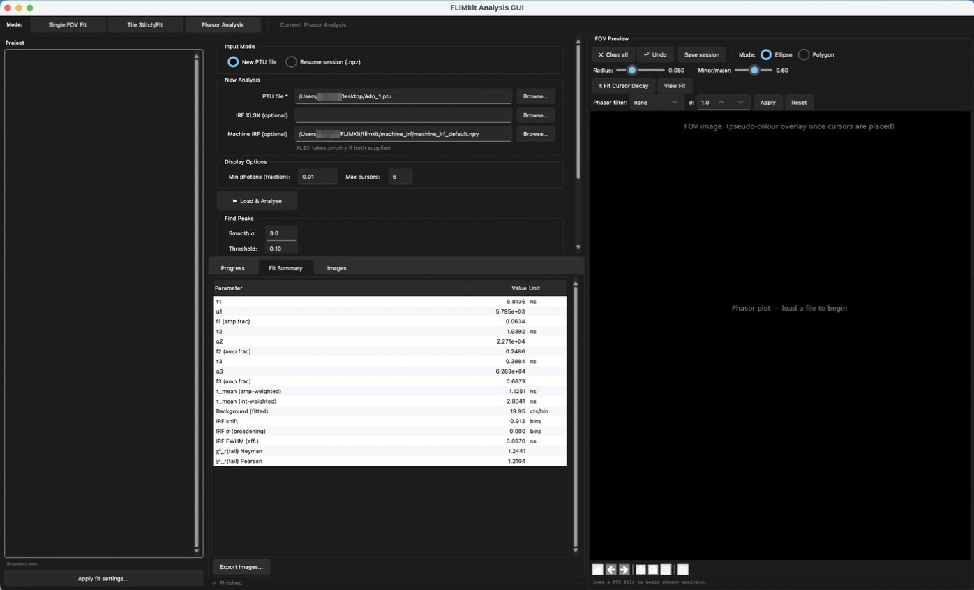
| Option | What it does |
|---|---|
| Input Mode: New PTU file / Resume session (.npz) | Start from a file, or reopen a saved phasor session with its cursors. |
| PTU file | The FLIM file. |
| IRF XLSX (optional) / Machine IRF (optional) | The calibration. Phasors need an IRF to place the universal circle correctly. The XLSX wins if both are given. |
| Min photons (fraction) | Pixels whose mean count per time bin is below this are left out of the plot. The default 0.01 is about 5 photons for a 529-bin decay. |
| Max cursors | How many cursors can be placed. |
| Load & Analyse | Computes and plots the phasor. |
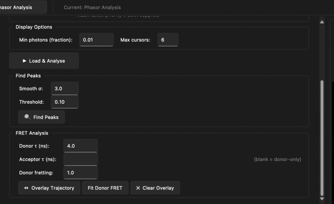
| Option | What it does |
|---|---|
| Find Peaks: Smooth σ, Threshold, Find Peaks | Smooths the phasor histogram and places cursors on the peaks above the threshold. |
| FRET Analysis: Donor τ, Acceptor τ, Donor fretting | The donor lifetime, an optional acceptor lifetime (blank for donor-only), and the fraction of donors that transfer. |
| Overlay Trajectory / Fit Donor FRET / Clear Overlay | Draw the FRET efficiency trajectory, fit it to the data, or remove it. |
On the plot, a click places an elliptical cursor and the matching pixels light up in the image above. The toolbar above the plot has Clear all and Undo, Save session, Ellipse or Polygon cursors, the Radius and Minor/major sliders for the cursor shape, and Fit Cursor Decay / View Fit to fit the summed decay of the pixels under a cursor.
Ado_1.ptu gave 48,357 valid pixels at 19.5 MHz. A cursor of radius 0.05 on the main cloud of the raw phasor took 6,259 pixels with a phase lifetime τ_φ of 2.20-2.71 ns (median 2.45 ns).
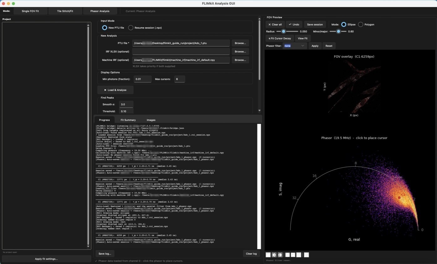
The raw cloud is wide because each pixel carries few photons. Phasor filter smooths the G and S coordinates in image space, which pulls the cloud together without changing where it sits:
| Filter | Parameter | What it does |
|---|---|---|
| none | Raw phasor. | |
| gaussian | σ | Gaussian smoothing of G and S. |
| median | size | Median filter of G and S. Removes outliers and keeps edges. |
| wavelet | Wavelet soft-thresholding (Daubechies db4). It takes no parameter. This is the filter closest to the LAS X phasor display. |
Apply runs the filter and Reset goes back to the raw data. With the wavelet filter and the same cursor, the count went to 13,771 pixels and τ_φ to 2.20-2.70 ns (median 2.43 ns).
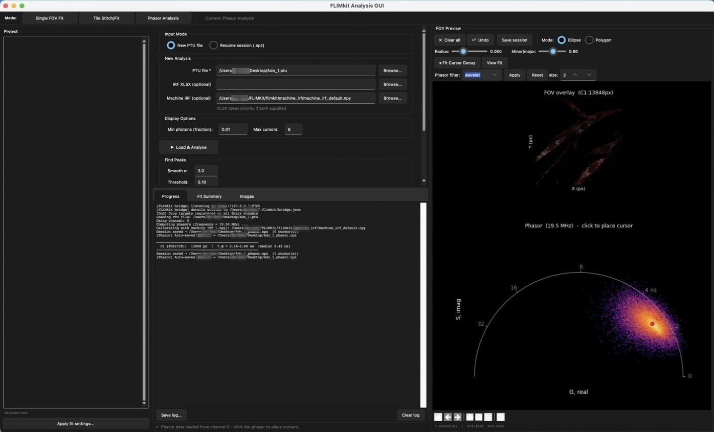
The phasor session is saved as <file>_phasor.npz next to the data whenever a cursor or the filter changes. Loading the same file again recomputes the phasor with the current IRF and then puts the saved cursors and filter back on it, the same way a fit session comes back, and the log says [Auto-Load] Restored 1 cursor(s) and the wavelet filter from Ado_1_phasor.npz. Clear all and Reset start again from nothing.
Step 13: Work from a project folder
A project is a folder of acquisitions. File > Open Project Folder... lists every FLIM file in it, groups region_zX slices into z-stacks and picks up .xlif files for tiles. It writes a project.json into the folder to remember them. For this I made a folder holding Ado_1.ptu, Ado_2.ptu and the eight slices Series008_z1.ptu to Series008_z8.ptu.
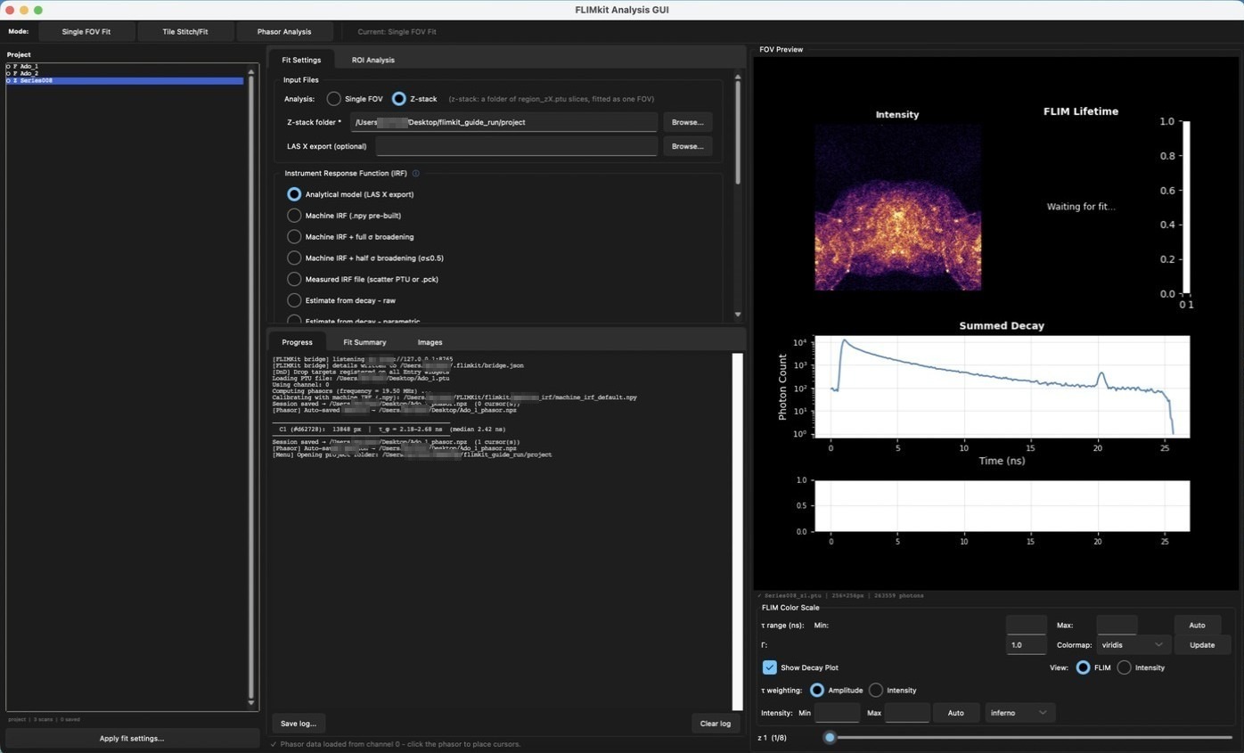
Each row shows a session mark (○ nothing saved, ● a fit, ◐ a phasor, ◉ both) and the scan type (F for a field of view, Z for a z-stack, T for tiles from an XLIF). The footer counts scans and saved sessions. Clicking a row loads it into the right form, restoring its fit and ROIs when there is a session.
To fit several files the same way, fit one, keep it selected, and press Apply fit settings... under the list.
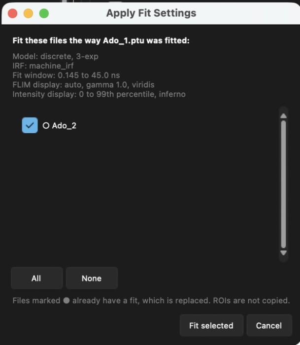
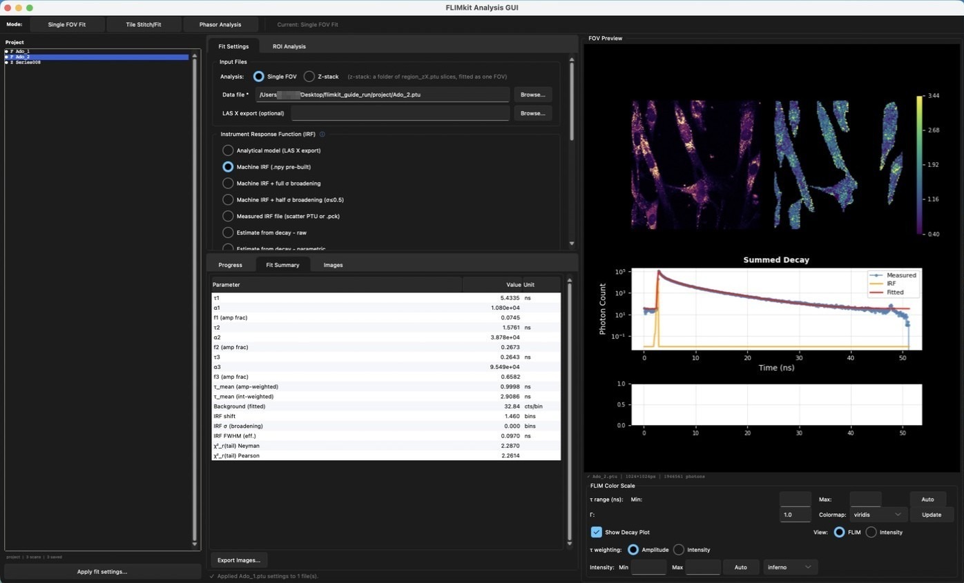
The dialog shows the model, IRF, lifetime bounds and display scales it will copy, and lists the other single-FOV files. Files that already have a fit are marked ● and their fit is replaced; ROIs aren't copied. I refitted Ado_1 in the project (3 components, machine IRF, cell mask, 8 x 8 binning) and applied it to Ado_2, which fitted to τ = 5.43, 1.58 and 0.264 ns with χ²_r(tail) = 2.29.
Clicking Ado_2 afterwards reloads its saved fit, residual plot included. The residuals are worked out from the saved decay and fitted curve. A session saved without the fitted curve has it rebuilt from the saved lifetimes, amplitudes, IRF shift and width and background, which gives back the same curve to rounding error.
Once two or more single-FOV files in the project have a fit, Export all... under the list exports them in one go. It has the same image, rendering and format options as the export dialog, and writes every file into one folder (exports in the project by default), each named after its scan. Each file is exported with its own saved display settings and ROIs. Two more boxes add each file's ROIs as <scan>_all_rois.geojson and its fit summary table as <scan>_fit_summary.txt, and a third adds the phasor plot and cursor image of every file that has a phasor session. A file with no ROIs gets no GeoJSON and a file with no phasor session gets no phasor PNGs, and the dialog at the end says which. Only fitted files are listed, so a file that has a phasor session but no fit isn't exported.
Step 14: Fit a z-stack
Selecting the Z row switches Analysis to Z-stack and fills the folder. The slider under the preview steps through the slices. The fit pools every slice to fit one set of lifetimes, then fits each slice per pixel with those lifetimes locked, so only the amplitudes change with depth (Timelapse and Z-stack Fitting). The form is the same as for a single FOV, and the button reads Run Z-stack Fit.
With the machine IRF and 2 components, the eight 256 x 256 slices (1,731,281 photons pooled) gave τ₁ = 3.48 ns and τ₂ = 0.572 ns, and per-slice amplitude-weighted means of 1.90-2.00 ns.
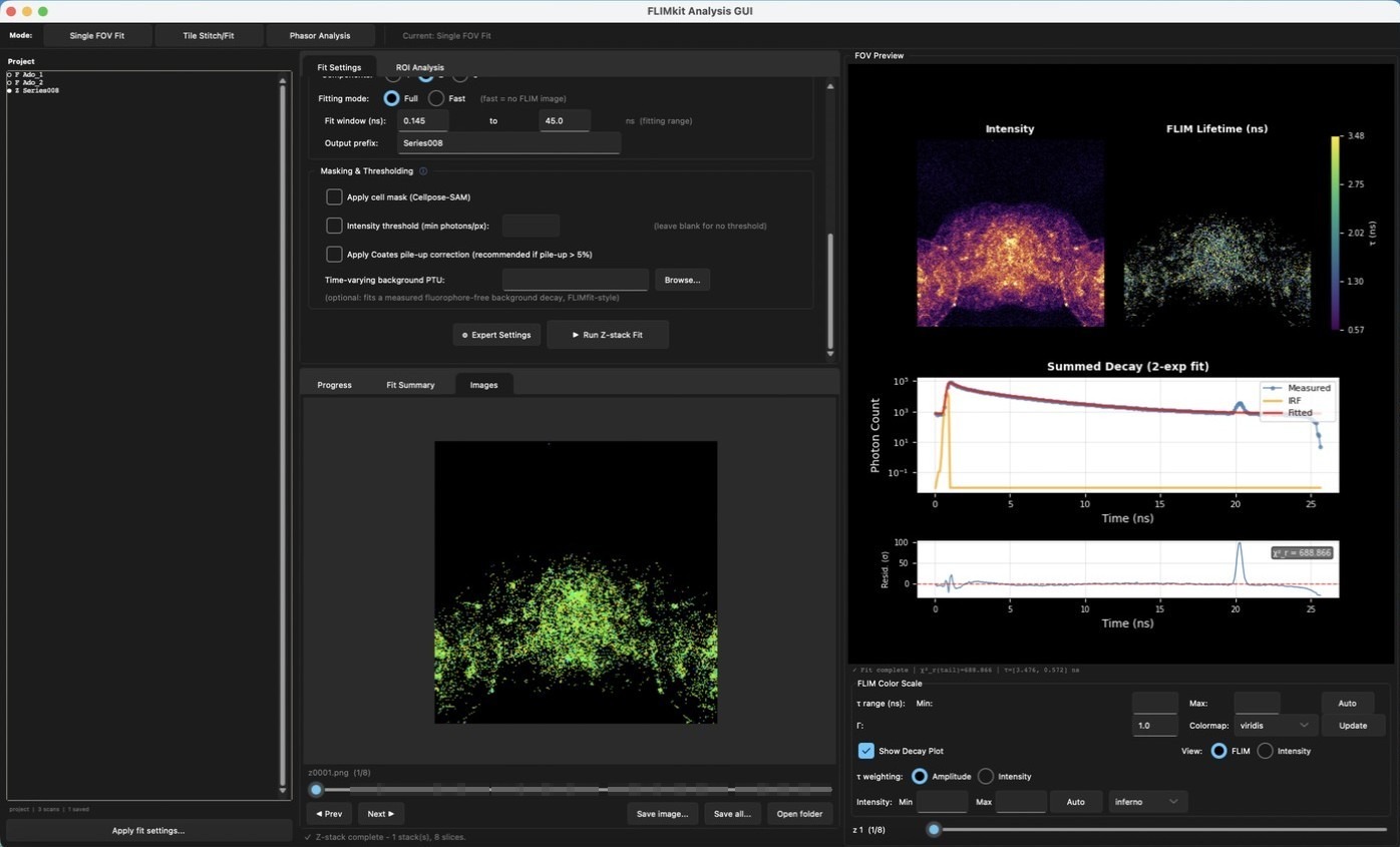
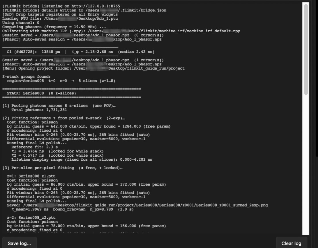
The residuals show why χ²_r(tail) came out at 688.9: this 25.7 ns period has a reflection peak at about 20 ns, and the whole period was fitted (bins 0-265).
Expert Settings apply to z-stacks the same way as to a single FOV. Setting Exclude bands to 19.6-21.2 dropped those bins from the fit, 248 of 265 fitted, and moved the pooled lifetimes to τ₁ = 3.66 ns and τ₂ = 0.604 ns. The calibrated tail χ² in Series008_reference_fit.json went from 159.6 to 21.1. It isn't near 1, so look at the residuals for what is left before trusting the absolute values. Spatial binning applies to every slice as well. The Images tab steps through the per-slice maps.
Step 15: Stitch tiles from an XLIF
Tile Stitch/Fit mode takes a tiled acquisition: the .xlif from the LAS X project's Metadata folder and the folder of PTU tiles exported with it.
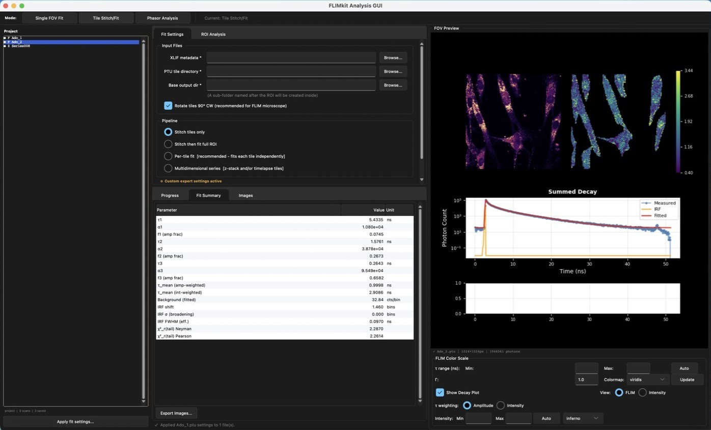
| Option | What it does |
|---|---|
| XLIF metadata | Tile positions and layout. |
| PTU tile directory | The folder of tiles. Tiles from several scans in one folder are sorted out by name. |
| Base output dir | A sub-folder named after the ROI is made inside it. |
| Rotate tiles 90° CW | Rotates each tile 90° clockwise before it is placed. On by default and recommended for Leica FLIM data. |
| Stitch tiles only | Registers and stitches the intensity image and the decay cube, without fitting. |
| Stitch then fit full ROI | Fits the whole mosaic at once. Needs tens of GB of RAM on large mosaics. |
| Per-tile fit | Fits a global decay for the lifetimes, then each tile with those lifetimes locked, and stitches the maps. The recommended option. |
| Multidimensional series | Per-tile fitting repeated over z and/or time, one stitched plane per (t, z) (Multidimensional Series). |
Below the pipeline choice come the same IRF, model and masking sections as for a single FOV, then:
| Option | What it does |
|---|---|
| Per-pixel fitting | Needed for the lifetime maps and for ROI analysis on the mosaic. |
| Export τ-weighted / intensity-weighted / amplitude-weighted map | 32-bit TIFF lifetime maps. |
| Save individual component maps | One TIFF per τᵢ. |
| Lifetime display / Intensity display | Display limits for the exported images. Blank is automatic. |
| Phase-correlation registration, Max shift (px) | Corrects stage drift before stitching (Tile registration). Raise the shift above 120 px if the drift is larger. |
| Pool decay every N timepoints | Multidimensional series only. Subsamples the files used for the pooled lifetime fit. |
| IRF XLSX dir | A folder with one <tile_name>.xlsx per tile. Blank uses the IRF method above. The machine IRF is safer, since per-tile exports vary. |
Step 16: What FLIMKit reads and writes
Files FLIMKit reads, apart from the FLIM data in Supported Input Formats:
| File | Where it's read | What it carries |
|---|---|---|
.xlsx, .csv, .tsv, .txt, .dat, .ascii, .asc |
LAS X export box, IRF XLSX, per-tile XLSX folder | The LAS X decay export: the IRF for the analytical model and the LAS X fit for comparison. |
.npy machine IRF |
Machine IRF path | The stored instrument response (Machine IRF Setup). |
Scatter .ptu or .pck |
Measured IRF file | A recorded IRF. |
Background .ptu |
Time-varying background PTU | A fluorophore-free decay fitted as background. |
.xlif (or .lif) |
Tile Stitch/Fit, project folders | Tile positions and layout. |
<file>.roi_session.npz |
Automatically when the file is opened, or File > Restore NPZ... | A saved fit, its ROIs, form settings and display scales. |
<file>_phasor.npz |
Phasor > Resume session | A saved phasor with its cursors. |
.geojson |
ROI Analysis > Import from GeoJSON, File > Import GeoJSON... | Regions from QuPath or any GeoJSON source. |
project.json |
File > Open Project Folder... | The project's scan list and output folder. |
Files FLIMKit writes:
| File | Written by | What's in it |
|---|---|---|
<prefix>_summed_<n>exp.png |
Every fit | Summed decay, IRF, fitted curve and residuals. |
<prefix>_pixelmaps_<n>exp.png |
Full fits | A figure of the per-pixel maps. |
<prefix>_lifetime_hist_<n>exp.png |
Full fits | Histogram of the per-pixel lifetimes. |
<prefix>_cell_mask.png |
Fits with the cell mask on | The Cellpose mask used. |
<file>.roi_session.npz |
Every fit, every ROI change, colour-scale changes | Fit results (summed and per-pixel arrays, decay, IRF, time axis, intensity, lifetime map), form settings, display scales and ROIs. Reopening the file restores all of it. File > Save NPZ / Save NPZ As... writes it on demand. |
<file>_phasor.npz |
Phasor mode, automatically, or Save session | Calibrated G and S before filtering, the mean intensity, frequency, the cursors (ellipses and polygons), their size and the filter applied. Restored when the file is loaded again. |
<scan>_intensity.png, <scan>_lifetime.png, <scan>_summed_decay.png |
Export Images..., PNG | The images as displayed, for slides. |
<scan>_intensity_colorbar.png, <scan>_lifetime_colorbar.png |
Export Images..., PNG, with the colour scale bar ticked | The preview's colour scales with their values. |
<scan>_phasor.png, <scan>_phasor_image.png |
Export Images... or Export all..., with the phasor box ticked | The phasor plot with its cursors, and the image coloured by cursor, each with a legend of cursor pixel counts and median τφ. |
<scan>_intensity.ome.tiff, <scan>_lifetime.ome.tiff |
Export Images..., OME-TIFF | Intensity as 32-bit photon counts, lifetime as 32-bit floats in ns with NaN where nothing was fitted, and the pixel size when known. |
<prefix>_*.tif |
Fits from fit_cli.py, batch, z-stack, timelapse, stitch and tile fits |
The intensity and lifetime maps, with the pixel size in the TIFF resolution tags, scaled for binning. |
<scan>.ome.zarr |
Export Images..., OME-Zarr | One compressed store, each image a channel, the fit summary in the metadata. |
ROI .csv |
Export as CSV, File > Export > Export ROI Table CSV | Per region: ID, name, type, τ mean/median/SD, photons and photon SD, and the per-ROI fit (τ_mean, χ²_r, τᵢ and αᵢ) when there is one. |
ROI .geojson |
Export as GeoJSON / Export All as GeoJSON, and the File > Export menu | Each region as a GeoJSON feature with its name, type, colour and statistics (τ median and SD, photons and SD). Self-intersecting outlines are repaired and flagged. Opens in QuPath. |
Fit summary .csv |
File > Export > Export Summed Fit CSV | The Fit Summary table. |
project.json |
Opening a project folder | Scan list, types, source paths and output folder. |
<stack>_reference_fit.json |
Z-stack fits | The pooled lifetimes, bounds, photons and slices used. |
<stack>_intensity_stack.npy, _tau_mean_amp_stack.npy, _alpha_<i>_stack.npy, _chi2_r_stack.npy, _calibrated_chi2_r_stack.npy |
Z-stack fits | (Z, H, W) arrays, one plane per slice. |
<stack>_zseries.csv / .json / .png |
Z-stack fits | Per-slice summary: mean amplitudes, mean τ and its SD, χ²_r and pixels fitted, with a plot. |
reference_decay.npz |
Z-stack fits | The pooled decay the reference lifetimes were fitted to. |
z0001/, z0002/, ... |
Z-stack fits | Per-slice fit plots and maps. |
Stitched .npy cube, intensity and τ TIFFs, CSV summary |
Tile Stitch/Fit and Batch ROI | See Tile stitching and fitting. |