 FLIMKit
Plugins / FLIMKit / Workflows · edit on GitHub
Workflows
Desktop GUI
python main.py
Five tabs. The right panel shows an FOV preview (intensity image + summed decay) for all fitting tabs, switching to the interactive phasor view when the Phasor tab is active.
Single PTU analysis
Open the GUI and select Single FOV Fit.
Go to Fit settings and fill in:
- PTU path: your
.ptufile. To get this from FLIM microscope software, open the lif/lof, go to the FLIM window, and export raw data. - IRF method: Machine IRF is recommended if you've built one. IRF XLSX works if you have a FLIM microscope software export for that specific PTU (right-click the summed/tail decay in the FLIM window → Export to Excel). Scatter PTU if you measured one directly. If none of those are available, use "Estimate from decay" and set FWHM to roughly 0.3-0.5 ns.
- Number of exponentials: 1, 2, or 3. Beyond 3 the math gets shaky and the biology harder to interpret, so that's the cap.
- Lifetime bounds: 0.145-45 ns by default. Adjust if you're working with unusually short or long lifetimes.
- Fitting mode: Full runs both summed and per-pixel fitting and is needed to generate the FLIM image in the UI. If you just want global lifetime values for the whole FOV, use FAST. Per-pixel fitting is slow, especially with more exponentials.
- Output prefix: defaults to the PTU filename in the PTU directory. Change it to keep outputs organised.
Masking and thresholding:
- Cell mask uses the Cellpose-SAM deep-learning segmentation model to isolate cell regions from background. It runs on GPU when available and falls back to CPU otherwise. The intensity image is percentile-normalised and resized to 224×224 before segmentation, then the label map is scaled back to the original resolution.
- Intensity threshold cuts out low-signal pixels from per-pixel fitting. Speeds things up and cleans up the map, but don't set it too high or you'll lose dim-but-real regions.
Expert fit settings (optimiser type, cost function, DE parameters) are under the Expert fit settings tab and are shared between single FOV and tile stitching pipelines.
Tile stitching and fitting
Open Tile Stitch / Fit.
You need the XLIF metadata file and the directory with the PTU tiles. The XLIF is in the Metadata folder of your FLIM microscope software project and contains stage coordinates and tile layout. If the directory has tiles from multiple scans mixed together, it should sort them out as long as the naming is consistent.
Pipeline modes:
- Stitch only builds a stitched intensity image and FLIM histogram cube, skips fitting. Exports the FLIM cube as an
.npyfile. Good for a quick visual check or if you want to hand the data off to something else. - Stitch then fit full ROI stitches everything into a single mosaic and fits it. Not recommended unless you have a capable machine and a small tile count, fitting a full mosaic requires a lot of RAM (tens of GBs) and is slow.
- Per-tile fit the recommended option for most cases. Builds a global decay from all tiles, runs an initial fit to get the lifetime components, then fits each tile separately using those fixed lifetimes. Results are stitched back together at the end. Same quality as fitting the mosaic directly, but far more memory-efficient.
- Multidimensional series per-tile fit repeated over a z and/or time axis, writing one stitched plane per
(t, z). Works with or without an XLIF. See Multidimensional Series.
Fitting parameters are the same as for single FOV. For tile work, the machine IRF is strongly recommended, per-tile XLSX IRFs from FLIM microscope software can vary across tiles and cause inconsistencies.
Per-pixel exports (when enabled):
- Intensity image (16-bit TIFF) total photon count per pixel
- α-weighted lifetime images (32-bit TIFF) amplitude or intensity-weighted τ maps with configurable display range
- Individual component τ maps (32-bit TIFF) spatial distribution per lifetime component
Tile registration:
The stage drifts during acquisition, so tiles need registration before stitching. Phase correlation is used in three passes:
- Column Y drift correction systematic Y drift across tile columns
- Row Y residual correction remaining per-row Y misalignment
- Row X backlash correction X misalignment from stage direction changes
You can set a maximum expected drift to help the algorithm. After registration, tiles are assembled using nearest-centre ownership: each output pixel is assigned to the tile whose centre is closest. Simple and fast, though sometimes not perfect at tile boundaries. Do check the stitched intensity image for any glaring misalignments.
Batch ROI fitting
Same settings as tile stitching, but no ROI analysis afterwards. Point it at a folder of XLIFs and it processes each one in sequence, outputting a CSV summary plus a folder per ROI with intensity images, decay arrays, and any lifetime exports you've selected.
ROI analysis
Available for single FOVs and single stitched ROIs. Place ROIs on the displayed FLIM image (rectangle, ellipse, polygon, or freehand) and get mean lifetime statistics per region.
ROIs are saved as part of the session. You can export them as GeoJSON for QuPath, the geometry and statistics travel with them. You can also import GeoJSON ROIs back in (from QuPath or anything else that writes GeoJSON), which makes it easy to define ROIs in one tool and analyse lifetimes in another. CSV export is available for spreadsheet-friendly output.
Note: GeoJSON import currently only preserves the outer boundary of shapes, donut-shaped ROIs with holes will lose the hole geometry on import.
Per-ROI decay fitting
The Fit ROI Decay button fits the summed decay from the selected region(s) independently, rather than using the whole-FOV fit.
Selecting regions: - Single region: click it in the list, then click Fit ROI Decay. - Multiple regions: Shift-click or Cmd-click to select several; they are combined into one union mask and treated as a single merged region for the fit.
Fit Options dialog: Before the fit runs, a small dialog appears pre-filled with the current global fit parameters. You can change any of the following without touching the main form:
| Option | Description |
|---|---|
| Components (n_exp) | 1-, 2-, or 3-exponential model |
| τ_min / τ_max (ns) | Lifetime search bounds |
| Cost function | Poisson deviance or Pearson χ² |
Click Run Fit to proceed or Cancel to abort.
Results window: Opens automatically after fitting. Shows: - Decay data (log-scale), IRF overlay, and fitted model curve - Weighted residuals panel with χ²_r annotation - Summary table: τ₁...τₙ, amplitudes A₁...Aₙ, amplitude-weighted τ_mean, χ²_r (tail)
Reopening results without refitting: Select the same region(s) and click View Fit. The last result for that selection is cached in memory and the plot window reopens instantly. The cache is lost when the app is closed.
Session persistence: After fitting, the numeric stats (τ_mean_fit, τ₁...τₙ, A₁...Aₙ, χ²_r) are written back into each region's statistics and saved to the .roi_session.npz automatically. The plot data (decay array, model curve) is not stored, so after reloading a session you need to refit to regenerate the plot - but the τ values are already there.
CSV export ("Export as CSV" button) includes all fit result columns: Tau_mean_fit_ns, Chi2_r_fit, and dynamic Tau1_fit_ns / Amp1_fit, Tau2_fit_ns / Amp2_fit, ... columns sized to the maximum number of exponential components across all fitted regions. Regions that haven't been fitted yet show N/A.
Phasor analysis
Load a PTU file plus an IRF calibration (XLSX, machine IRF, etc). The app computes the phasor histogram and shows it alongside the intensity image. Click on the phasor plot to place elliptical cursors, the corresponding pixels in the intensity image highlight immediately.
Per-cursor stats (phase lifetime τ_φ, pixel count, 5th-95th percentile range) print to the progress log. With two or more cursors, a two-component decomposition line is drawn between them and the component lifetimes and mean fractions are reported.
Sessions save to .npz allowing you to come back later and pick up where you left off.
Phasor panel controls:
- Clear all / Undo: remove everything or step back one cursor at a time
- Save session: writes phasor arrays + cursor state to
.npz - Radius / Minor:major sliders: resize the cursor in real time; stats update immediately
Spatial filtering:
A filter row sits above the cursor controls. Select a method, set parameters, and click Apply. Reset restores the original unfiltered data.
| Method | Parameter | Description |
|---|---|---|
gaussian |
σ (0.5-10 px) | Gaussian smoothing via phasorpy's NaN-aware implementation |
median |
size (3-15 px, odd) | Median filter; removes outlier pixels while preserving edges |
wavelet |
none | Wavelet soft-thresholding (Daubechies db4, MAD noise estimator) |
Filtering is applied in phasor space (G and S coordinates) after calibration. The phasor plot and cursor stats update immediately after applying.
Guided Terminal UI (main.py)
python main.py --cli
| Option | Description |
|---|---|
| FLIM FIT a single FOV | Loads a PTU, builds an IRF, runs summed and/or per-pixel fitting |
| Phasor analysis | Opens the interactive phasor cursor tool |
| Reconstruct a FOV and FLIM FIT | Stitches multi-tile PTU data from XLIF metadata then fits the mosaic |
| Just stitch multiple tiles together | Tile stitching only, intensity images and FLIM histogram cubes |
| Timelapse batch fit | Fits a time series of PTUs as one FOV with a shared reference lifetime |
| Z-stack batch fit | Fits an axial stack of region_zX.ptu slices as one FOV |
| About | Version info and roadmap |
Machine IRF Setup (Required)
The machine IRF is a calibrated instrument response built from your specific microscope configuration. Build it once per system/session setup and reuse it. This is the most reliable IRF method and the one I'd recommend over any of the XLSX-based alternatives. It stores the full shape instead of recreating one from a few datapoints. It isnt perfect and an actual recorded IRF will always be ideal, but it's a big step up from trying to estimate the IRF or relying on the sometimes spotty XLSX IRF exports.
You need matched .ptu + .xlsx pairs. The more the better, but 10-20 is generally sufficient.
| Goal | Minimum pairs |
|---|---|
| Peak-placement only | 4-6 |
| Stable IRF shape + placement | 10-12 |
| Robust production use | 15-20 |
Don't go below 10 unless your data is very homogeneous.
GUI method
- Open the GUI, go to Machine IRF Builder
- Select your pairs folder
- Keep anchor as
peakand reducer asmedianunless you have a reason to change them - Build and save as
machine_irf_default
Save locations:
| Context | Location |
|---|---|
| Running from source | flimkit/machine_irf/ |
| Compiled app (macOS/Linux) | ~/.flimkit/machine_irf/ |
| Compiled app (Windows) | C:\Users\<name>\.flimkit\machine_irf\ |
To use an IRF kept somewhere else, a shared drive or one per microscope for example, set it in File > Preferences... > Files > Default machine IRF (.npy). Browse picks the file, Use the built-in IRF clears the setting, and Save checks the file loads before accepting it. The choice is stored in ~/.flimkit/config.json, so it applies to every form straight away and stays set after a restart. The terminal tools read the same setting. If the chosen file later goes missing, FLIMKit says so in the log and falls back to the built-in one.
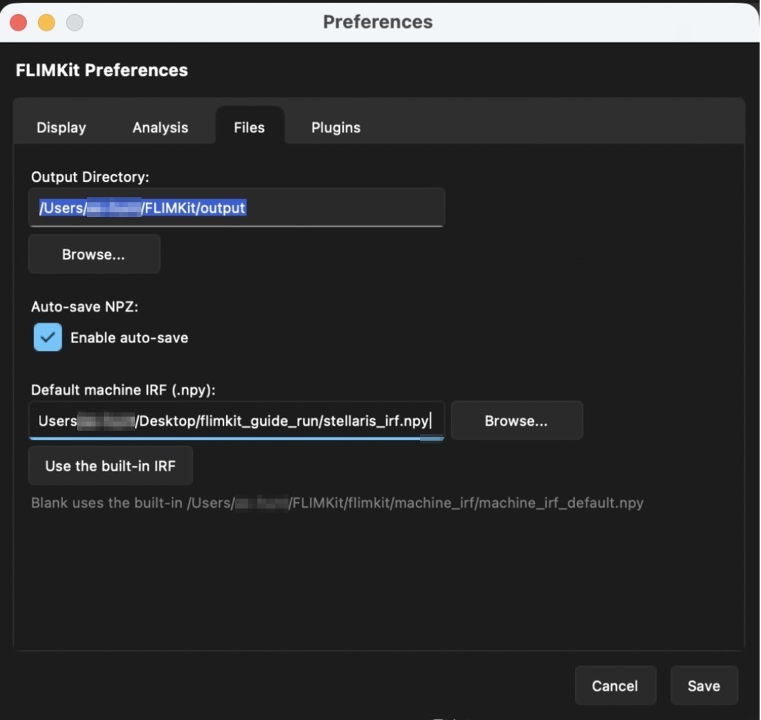
A newly built machine_irf_default is picked up after a restart, unless a different default is set in Preferences.
Python API
from flimkit.FLIM.irf_tools import build_machine_irf_from_folder

build_machine_irf_from_folder(
    folder="/path/to/pairs",
    align_anchor="peak",
    reducer="median",
    save=True,
    output_name="machine_irf_default",
)
FLIM Reconvolution Fitting (CLI)
python fit_cli.py [OPTIONS]
Required
| Argument | Description |
|---|---|
--ptu PATH |
Path to the PTU file |
IRF Arguments
| Argument | Description |
|---|---|
--machine-irf PATH |
Pre-built machine IRF .npy file (recommended) |
--irf PATH |
Scatter PTU for a directly measured IRF |
--irf-xlsx PATH, --irf-export PATH |
LAS X .xlsx or delimited text export (.csv, .tsv, .txt, .dat, .ascii, .asc) for analytical IRF fitting |
--xlsx PATH, --analysis-export PATH |
LAS X .xlsx or delimited text export for comparison |
--no-xlsx-irf |
Use the analysis export for comparison only; don't use its IRF |
--estimate-irf {raw,parametric,machine_irf,machine_irf_sigma_full,machine_irf_sigma_half,none} |
Estimate IRF from decay rising edge, or reuse the machine IRF shape (default: none) |
--irf-fwhm FLOAT |
IRF FWHM in ns |
--irf-bins INT |
Number of bins for the IRF (default: 21) |
--irf-fit-width FLOAT |
Region around time zero for IRF fitting in ns (default: 1.5) |
IRF priority order (highest to lowest):
1. --machine-irf
2. --irf (scatter PTU)
3. --irf-xlsx
4. --xlsx IRF columns (unless --no-xlsx-irf)
5. --estimate-irf raw / parametric
6. Gaussian fallback from FWHM
Fitting Arguments
| Argument | Description |
|---|---|
--nexp {1,2,3} |
Number of exponential components (default: 3) |
--tau-min FLOAT |
Minimum lifetime bound in ns (default: 0.145) |
--tau-max FLOAT |
Maximum lifetime bound in ns (default: 45.0) |
--mode {summed,perPixel,both} |
Fitting mode (default: both) |
--binning INT |
Spatial binning for per-pixel fitting (default: 1) |
--min-photons INT |
Minimum photons per pixel (default: 10) |
--optimizer {lm_multistart,de} |
Optimiser for summed fit (default: de) |
--restarts INT |
LM multi-start restarts (default: 8) |
--de-population INT |
DE population size (default: 30) |
--de-maxiter INT |
DE maximum iterations (default: 5000) |
--workers INT |
CPU cores for DE (-1 = all; auto-limited to 1 in compiled app) |
--no-polish |
Skip LM polish step after DE |
--bootstrap INT |
Resampled refits for the bootstrap ± errors (default: 25, 0 turns them off) |
--cost-function {poisson,chi2} |
Cost function (default: poisson) |
--fit-start-ns FLOAT |
Fit window start in ns (default: auto from IRF onset) |
--fit-end-ns FLOAT |
Fit window end in ns (default: auto) |
--exclude-ns SPEC |
Bands to drop from the fit, e.g. "7.2-8.8" or "7.2-8.8,11.0-11.5". See Fit window and exclusion bands |
--correct-pileup |
Apply Coates pile-up correction to the decay before fitting |
--free-tau |
Let lifetimes float per pixel instead of locking them to the summed fit |
--intensity-threshold INT |
Minimum photons per pixel mask |
--tau-display-min FLOAT |
Min lifetime for exported tau images (ns) |
--tau-display-max FLOAT |
Max lifetime for exported tau images (ns) |
--tvb-ptu PATH |
Reference PTU of a fluorophore-free background (buffer / culture-medium well). Its summed decay is fit as a scaled time-varying background V·b(t) instead of a flat offset (FLIMfit-style). |
--tvb-channel INT |
Detector channel for --tvb-ptu (default: same as --channel) |
Time-varying background correction
By default the fit treats the baseline as a flat constant Z. When a sample has structured background (autofluorescence from the medium, scatter, plate fluorescence), that background has its own decay shape, and a flat offset cannot remove it. Pass --tvb-ptu with a measurement of a fluorophore-free region and FLIMKit fits the full model B = V·b(t) + Z, where b(t) is the normalized measured background profile and V is a non-negative scale recovered per fit (and per pixel). The same option is available in the GUI (the "Time-varying background PTU" picker on the Single-FOV, Batch and Tile-Stitch panels) and the Python API (tvb_profile= / fit_tvb= on fit_summed, fit_per_pixel, and the distribution variants). The per-pixel scale is written out as a *_tvb_scale.tif map.
Output Arguments
| Argument | Description |
|---|---|
--out NAME |
Output file prefix (default: flim_out, anchored to PTU directory) |
--no-plots |
Suppress plot generation |
--channel INT |
Detection channel (default: auto-detect) |
Timelapse and Z-stack Fitting
Both fit a stack of PTUs as a single field of view: all slices are pooled to fit one shared reference lifetime, then each slice is fitted per-pixel with τ locked, so lifetime is held constant across the stack while amplitude and intensity vary. Timelapse uses time as the stack axis, z-stack uses depth. They share the same code path (flimkit/FLIM/batch.py).
Reach them from the terminal UI (python main.py --cli → "Timelapse batch fit" / "Z-stack batch fit"), from the GUI (the Analysis toggle next to the input file in the Single FOV tab switches to Z-stack), or programmatically:
from flimkit.interactive import timelapse_flim_fit, zstack_flim_fit

zstack_flim_fit()      # parses sys.argv
timelapse_flim_fit()
Expected filename patterns: region_tX[_sY][_zZ].ptu for timelapse, region_zX.ptu for a z-stack (as exported in Leica .sptw workspaces).
| Argument | Description |
|---|---|
--ptu-dir PATH |
Folder of stack PTUs (required) |
--output-dir PATH |
Base output directory (required) |
--ref-tau1 FLOAT |
Reference τ₁ in ns; skips the pooled global fit |
--ref-tau2 FLOAT |
Reference τ₂ in ns; required alongside --ref-tau1 when --nexp ≥ 2 |
--fit-start-ns FLOAT |
Fit window start in ns (default: auto from IRF onset) |
--fit-end-ns FLOAT |
Fit window end in ns (default: auto) |
--exclude-ns SPEC |
Bands to drop from the fit, e.g. "7.2-8.8" or "7.2-8.8,11.0-11.5" |
--correct-pileup |
Coates pile-up correction |
--binning INT |
Spatial binning (NxN) before the per-slice per-pixel fit (default: 1) |
--no-stack |
Skip saving the (T,H,W) / (Z,H,W) map stacks |
--bound-fraction |
Z-stack only: compute bound fraction α₂/(α₁+α₂) |
--nexp, --tau-min, --tau-max, --machine-irf, --estimate-irf, --irf-fwhm, --irf-bins, --irf-fit-width, --optimizer, --restarts, --de-population, --de-maxiter, --workers, --no-polish, --channel, --min-photons, --cost-function and --no-plots behave as in fit_cli.py.
Outputs land under output-dir in one folder per group: per-slice amplitude/intensity/lifetime maps, the pooled reference fit as *_reference_fit.json, stacked maps, and a series summary as *_zseries.csv / .json / .png (*_timeseries.csv for timelapse).
These treat each _sY position as an independent field of view. If the positions are overlapping tiles of one larger region, use the multidimensional series fit below instead, which stitches them.
Multidimensional Series (stitched tiles over z and time)
For tiled acquisitions with a z and/or time axis, where the tiles overlap and should be stitched into one canvas per plane rather than fitted as separate fields of view.
Stitch tab → pipeline "Multidimensional series".
Tile positions are found by maximising the correlation between neighbouring tiles over candidate shifts. FFT phase correlation is not used, because on real mosaics with ~10% overlap it returns no distinguishable peak.
Give it an XLIF or LIF if you have one and it is used as the starting layout, then refined against the overlap. The refinement is not optional: on the test set the metadata put both tiles at the same y while the images show a 23 px offset, which is the difference between an overlap correlation of 0.77 and 0.04. Metadata still helps for more than two tiles, where chaining pairwise shifts can drift. With no metadata the positions come from the overlap alone, which needs structure in the overlap to match on and is unreliable on sparse or thin samples.
One pooled decay is fitted across the whole series, and every plane is then fitted per-pixel with those τ values locked, so amplitudes stay comparable between timepoints. "Pool decay every N timepoints" subsamples that pooling step, which only needs photon statistics rather than every file.
Filenames follow the same region_tX[_sY][_zZ].ptu convention as the timelapse fit, and at least two positions are required.
from flimkit.formats.PTU.stitch import fit_flim_series

manifest = fit_flim_series(ptu_dir, output_dir, args, pool_stride=10)
Outputs are one directory per (t, z) plane, each holding the usual fitted maps, plus a *_series_index.json manifest recording the recovered tile positions, the consensus τ values and every plane written. Tile positions can be supplied directly as tile_positions= to skip recovery.
Registration quality is reported as a correlation per tile pair. A low value means the overlap was not found, usually because the tiles genuinely do not overlap or the region is too sparse to register; supply positions from a .lif or .xlif in that case.
Fit window and exclusion bands
Available on fit_cli.py, timelapse and z-stack alike. By default the fit spans the decay from the IRF onset to the end of the record. Two things break that: signal before the rise (IRF artefacts) and reflection peaks partway down the tail, which pull a multi-exponential fit toward a spurious short component. --fit-start-ns and --fit-end-ns set the window explicitly; --exclude-ns drops one or more bands inside it, given as comma-separated lo-hi pairs in ns.
--fit-start-ns 0.5 --fit-end-ns 12.0 --exclude-ns "7.2-8.8"
Excluded bins are removed from the cost function rather than zeroed, so the fit statistic stays comparable.
On a synthetic 3.5 ns decay with a 5% reflection planted at 8.0 ns, excluding 7.5-8.5 moves the recovered lifetime from 3.5676 ns to 3.4872 ns and χ²_r from 8.33 to 0.73.
In the Python API the controls are fit_start_ns=, fit_end_ns= and exclude_ns= on fit_summed, where exclude_ns takes a list of (lo, hi) tuples; flimkit.interactive.parse_exclude_ns converts the string form. fit_per_pixel instead takes the resolved bin set as fit_idx=, which fit_summed reports back in its summary:
popt, summary = fit_summed(..., exclude_ns=[(7.5, 8.5)])
maps = fit_per_pixel(..., fit_idx=summary['fit_idx'])
The GPU backends honour the window too. All four per-pixel kernels take fit_idx and restrict themselves to it, so excluding a reflection peak does not cost the GPU.
Synthetic Data Generation (CLI)
Generates FLIM data with a known ground truth: a sample PTU, a matching IRF PTU, and a JSON file recording the parameters used. Intended for cross-software validation, where the same file is fitted in FLIMKit and elsewhere and the recovered lifetimes are compared against truth.
python synth_cli.py --out ./validation --tau 3.0,0.8 --amps 0.7,0.3 --photons 1e5
| Argument | Description |
|---|---|
--out PATH |
Output directory for the PTUs and truth JSON (required) |
--name NAME |
Base name for the files (default: synth) |
--tau SPEC |
Lifetime(s) in ns, comma-separated for multi-exponential (default: 4.1) |
--amps SPEC |
Amplitudes for multi-exponential τ, comma-separated (default: equal) |
--photons SPEC |
Summed photon count; comma-separated generates a series, e.g. "2e4,1e5,5e5" (default: 1e5) |
--period-ns FLOAT |
Laser period in ns, sets the sync rate (default: 50.0) |
--res-ps FLOAT |
TCSPC bin width in ps (default: 25.0) |
--irf-fwhm-ns FLOAT |
IRF FWHM in ns (default: 0.15) |
--irf-center-ns FLOAT |
IRF peak position in ns (default: 2.0) |
--reflection-ns FLOAT |
Plant a reflection peak at this time in ns, e.g. 8.0 |
--reflection-frac FLOAT |
Reflection intensity as a fraction of total signal (default: 0.02) |
--reflection-width-ns FLOAT |
Reflection peak FWHM in ns (default: 0.15) |
--pileup-pp FLOAT |
Apply pile-up at this many photons per pulse, e.g. 0.1 |
--background-frac FLOAT |
Flat background as a fraction of total signal (default: 0.0) |
--image INT |
Image side length in pixels, square (default: 16) |
--no-irf |
Skip writing the IRF PTU |
--sdt |
Also write Becker & Hickl .sdt versions of sample and IRF |
--reflection-ns pairs with --exclude-ns on the fitting side: plant a reflection at a known position, then confirm that excluding that band recovers the input lifetime.
Phasor Analysis (CLI)
python phasor_cli.py [OPTIONS]
| Argument | Description |
|---|---|
--ptu PATH |
Path to a .ptu file |
--irf PATH |
IRF calibration Excel file (XLSX) |
--machine-irf PATH |
Machine IRF .npy file |
--session PATH |
Resume a saved .npz session |
With no arguments, the CLI drops into a guided inquirer flow.
Python API
Phasor Analysis
from flimkit.phasor_launcher import launch_phasor, save_session, load_session

# Interactive prompts
state = launch_phasor()

# Pass paths directly
state = launch_phasor('data.ptu', irf_path='irf.xlsx')

# With spatial phasor filtering
state = launch_phasor('data.ptu', irf_path='irf.xlsx',
                      phasor_filter='gaussian', filter_kwargs={'sigma': 1.5})
state = launch_phasor('data.ptu', irf_path='irf.xlsx',
                      phasor_filter='median',   filter_kwargs={'size': 5})
state = launch_phasor('data.ptu', irf_path='irf.xlsx',
                      phasor_filter='wavelet')

# Resume a saved session
state = launch_phasor(session_path='session.npz')

# Save/load programmatically
save_session('session.npz',
             real_cal=state['real_cal'], imag_cal=state['imag_cal'],
             mean=state['mean'], frequency=state['frequency'],
             cursors=state['cursors'], params=state['params'])

sess = load_session('session.npz')

# Save a session's phasor plot and cursor image as PNGs
from flimkit.phasor.export import savePhasorPlots
savePhasorPlots(load_session('data_phasor.npz'), 'exports', 'data')
PTU File Reading
from flimkit.formats.PTU.reader import PTUFile

ptu = PTUFile('data.ptu', verbose=True)
decay = ptu.summed_decay(channel=None)           # auto-detect channel
stack = ptu.pixel_stack(channel=None, binning=1) # (Y, X, H)
print(ptu.n_bins, ptu.tcspc_res, ptu.time_ns)
Signal Extraction (xarray)
from flimkit.formats.PTU.tools import signal_from_PTUFile
import numpy as np

signal = signal_from_PTUFile('data.ptu', dtype=np.uint32, binning=4)
# signal.attrs['frequency'] - modulation frequency in MHz
Phasor Computation
from flimkit.phasor.signal import (
    return_phasor_from_PTUFile,
    get_phasor_irf,
    calibrate_signal_with_irf,
    calibrate_signal_with_machine_irf,
)

mean, real, imag = return_phasor_from_PTUFile('data.ptu')

# Calibrate with XLSX IRF
irf_time_ns, irf_counts = get_phasor_irf('irf.xlsx')
real_cal, imag_cal = calibrate_signal_with_irf(
    signal, real, imag, irf_time_ns, irf_counts, frequency)

# Calibrate with machine IRF
real_cal, imag_cal = calibrate_signal_with_machine_irf(
    signal, real, imag, 'machine_irf_default.npy', frequency)
Tile Stitching
from flimkit.formats.PTU.stitch import stitch_flim_tiles, load_flim_for_fitting
from pathlib import Path

result = stitch_flim_tiles(
    xlif_path=Path('metadata/R 2.xlif'),
    ptu_dir=Path('PTU_tiles/'),
    output_dir=Path('stitched/R_2/'),
    ptu_basename='R 2',
    rotate_tiles=True,
)

stack, tcspc_res, n_bins = load_flim_for_fitting(
    Path('stitched/R_2/'), load_to_memory=True)
decay = stack.sum(axis=(0, 1))
Intensity Images & Cell Masking
from flimkit.image.tools import (
    make_intensity_image, make_cell_mask,
    apply_intensity_threshold, pick_intensity_threshold,
)

intensity = make_intensity_image('data.ptu', rotate_90_cw=True)
mask      = make_cell_mask(intensity, save_mask=True, path='output/')
int_mask  = apply_intensity_threshold(intensity, threshold=50)
threshold = pick_intensity_threshold(intensity)  # interactive slider